This is a guest blog entry by Fotios Petropoulos.
A few months ago, Bergmeir, Hyndman and Benitez made available a very interesting working paper titled “Bagging exponential smoothing methods using STL decomposition and Box-Cox transformation”. In short, they successfully employed the bootstrap aggregation technique for improving the performance of exponential smoothing. The bootstrap technique is applied on the remainder of the series which is extracted via STL decomposition on the Box-Cox transformed data so that the variance is stabilised. After generating many different instances of the remainder, they reconstruct the series by its structural components, ending with an ensemble size of 30 series (the original plus 29 bootstraps). Using ETS (selecting the most appropriate method from the exponential smoothing family using information criteria) they produce multiple sets of forecasts, for each one of these series. The final point forecasts are produced by calculating the arithmetic mean.
The performance of their approach (BaggedETS) is measured using the M3-Competition data. In fact, the new approach succeeds in improving the forecasts of ETS in every data frequency, while a variation of this approach produced the best results for the monthly subset, even outperforming the Theta method. I should admit that the very last bit intrigued me even more to search in depth how this new approach works and if it is possible to improve it even more. To this end, I tried to explore the following:
- Is the new approach robust? In essence, the presented results are based on a single run. However, given the way bootstrapping works, each run may give different results. Also, what is the impact of the ensemble size (number of bootstrapped series essentially) on the forecasting performance? A recent study by the owner of this blog suggests that higher sample sizes result in more robust performance in the case of neural networks. Is this also true for the ETS bootstraps?
- How about using different combination operators? The arithmetic mean is only one possibility. How about using the median or the mode (both have shown increased performance in the aforementioned study by Nikos – a demonstration of the performance of the different operators can be found here).
- Will the new approach work with different forecasting methods? How about replacing the ETS with ARIMA? Or even Theta method?
To address my thoughts, I set up a simulation, using the monthly series from the M3-Competition. For each time series, I expanded the number of bootstrapped series to 300. Then, for every ensemble with sizes from 5 up to 150 members with step 5, I randomly selected the required number of bootstrapped series as to create 20 groups. The point forecasts for each group were calculated not only by the arithmetic mean but also by the median. For each operator and for each ensemble size considered, a five-number summary (minimum, Q1, median, Q3 and maximum sMAPE) for the 20 groups is graphically provided in the following figure.

So, given that the ensemble size is at least of size 20, we can safely argue that the performance of the new approach is 75% of the times better than that of Theta method (and by far always better than that of ETS). Having said that, the higher the number of bootstraps, the better and more robust the performance of the new approach is. This is especially evident for the median operator. Another significant result is that the median operator performs better at all times compared to the mean operator. Both results are in line with the conclusions of the aforementioned paper.
In addition, I repeated the procedure using the Theta method as the estimator. The results are presented in the next figure.
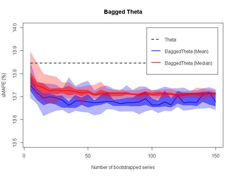
Once more, the new approach is proved to be better than the estimator applied only on the original data. So, it might be of value to check whether this particular way of creating bootstrapped time series is something that can be generalised, so that the new approach can be regarded as a “self-improving mechanism”. However, it is worth mentioning that in this case the arithmetic mean operator generally performs better than that of the median operator (at least with regards to the median forecast error), resulting, though, in more variable (less robust) performance.
By comparing the two figures, it is interesting that BaggedETS is slightly better than BaggedTheta for the ensemble sizes greater than 50. But this comes with a computational cost: BaggedETS is (more or less) 40 times slower in producing forecasts compared to BaggedTheta. This may render the application of BaggedETS problematic even for a few thousands SKUs if these are to be forecasted daily.
To conclude, I find that the new approach (BaggedETS) is a very interesting technique that results in improved forecasting performance. The appropriate selection of the ensemble size and the operator can lead to robust forecasting performance. Also, one may be able to use this approach with other forecasting methods as well, as to create the BaggedTheta, BaggedSES, BaggedDamped, BaggedARIMA…
Fotios Petropoulos (October 31, 2014)
Acknowledgments
I would like to thank Christoph Bergmeir for providing clarifications on the algorithm that rendered the replication possible. Also, I am grateful to Nikos for hosting this post in his forecasting blog.
Update 13/11/2014: Minor edits/clarifications by Fotis.
Thank you for this excellent post. What bootstrapping procedure was used for this simulation exercise? Can you please share the methedology ?
Many Thanks
The bootstrap is done using the following steps:
1. Box-Cox transformation is applied to the series.
2. The time series is separated into its components using STL decomposition.
3. The residuals of the decomposition are bootstrapped using moving block bootstrap. The block is twice the sampling frequency of the series.
4. Recompose the series from the trend and seasonal components from the STL decomposition and the bootstrapped residuals.
5. Inverse the Box-Cox transformation.
More details can be found in the working paper by Bergmeir et al., which can be downloaded here.
The working paper, by Bergmeir et al. mentions a small modification for monthly series.
5. ets() forecast.
6. Inverse the Box-Cox transformation, and apply de mean.
This modification improves the rest of algorithms (table on page 16).
I was wondering your opinion about to use this aproach for monthly series.
Thanks
Thansk. A very interestin post.
Do you try BaggedMAPA?
This is a very interesting suggestion. My first feeling is that BaggedMAPA would help MAPA in forecasting performance but not as much as in the case of ETS. The reason is that MAPA already tackles the model uncertainty by combining forecasts derived from multiple frequencies. See also Nikos’ and mine recent discussion (now published in Foresight practitioners’ journal): http://kourentzes.com/forecasting/2014/05/26/improving-forecasting-via-multiple-temporal-aggregation/
In any case, I will run some additional experiments and check if my assumption holds. But this might take some time. The first figure provided in this post is the result of 1428×300 > 400K fits of ETS. Applying the MAPA on the same design translates to forecasting 1428x300x12 > 5M time series using the ETS function.
It is useful of course to keep in mind that several of the additional fits of MAPA would be done at series of lower frequency and therefore much faster! An interesting experiment to try.
Thanks Fotios. It is a great valuable job.
Another question, I ask myself: Do you apply “bootstrap algorithm” before dividing time series into multiple frequencies or after.?
Thanks again.
If we were to retain the original motivation of MAPA then the bootstrapping should be done before aggregating the time series into multiple frequencies. However, as both MAPA and bootstrapping provide similar benefits in terms of model selection/parameterisation I would not expect substantial differences. Given the current implementation of MAPA in R bootstrapping before MAPA would be the easiest to do as well.
Actually this is an interesting point. My first feeling is what Nikos suggests: first bagging then MAPA. But it would be interesting to examine if first MAPA then bagging would give different insights.
In any case, the first experiment (first bagging then MAPA) is now running but it will take some more days to finish – so STAY TUNED!
Thank you. I hope the results 🙂
Anything interesting about the experiment.?
Many thanks,
Hi Nikos and Fotios, when I run the basic ets on M3 monthly dataset I get 14.28 as sMAPE. Can you please let me know what do you get for sMAPA for ets in the first figure ?
Also for theta I get 13.83 in sMAPE when applied to the M3 monthly, I get get 13.835, can you please let me know what is the sMAPE in the second figure for basic theta model ?
Many Thanks
For ETS, I get sMAPE=14.286% with forecast package versions 5.5 or 5.6 (v5.5 was used for this post).
For Theta, I am using my own implementation (not yet publicly available), where I get sMAPE=13.845%.
Thanks so much Fotios. For bootstraping time series, I used tsboot in boot package in R. Can you please let me know what function/method you used for bootstraping time series ?
Thanks
I am not using the boot package at all. I am using the R functions BoxCox.lambda(), BoxCox() and stl() to extract the remainder, which is the vector to be bootstrapped. To this end, I have implemented from scratch a moving block bootstrap function, based on the description provided by Bergmeir et al. (http://robjhyndman.com/working-papers/bagging-ets/). Once the bootstrap of the remainder has been calculated, the series is recomposed and inversed using the InvBoxCox() function. Lastly, each bootstrapped series is extrapolated using the ets() function.
Thanks Fotios, this procedure seems to be computationally very expensive. It took me whopping ~22 hours to run full ETS. I really like your charts much better than the point estimates. May be na aive question, should the Q1,Q3, Min and Max in the 5 point summary same for both mean and median operator ? Shold the mean and median are two metrics should change ? In the charts above I see the Q1/Q3/Min/Max for mean and median operator separately. Thanks for clarifications.
Fotios, never mind, I got the 5 point summary at each ensemble size. Please correct me if my interpretation below is correct:
A. Create 300 bootstrapped time series.
B. For Mean operator do the following:
1. Choose an ensemble size n from ( n = 5,10,15,….150)
2. For each ensemble size selected, randomly draw “n” samples from step A and estimate ETS predictions for each sample.
3. Average Predictions from individual sample.
4. Calcuate sMAPE
5. Repeat step 2,3 and 4, 20 times for each ensemble size n.
6. Report 5 point summary i.e., median,min,max,Q1 and Q3 from step 5 of sMAPE.
Repeat the same for median operator (step 3 above).
Biz_Forecaster your description looks fine to me. I noticed that in step 5 you repeated each step 20 times for each ensemble size, following Fotios’ description. I wonder if you could use more, so as to sample the distribution of the combined predictions better. This should make the shape of the quantiles smoother across different ensemble sizes. I would be especially interested in exploring any non-normalities of the sMAPE distribution for various ensemble sizes. What is the distribution like and is it the same across different ensemble sizes?
Biz_Forecaster: Your procedure seems correct. However, I do forecast all 300 bootstraps before making combinations, so that I save some computations (in essence, some bootstraps are used again and again).
Then, what you describe is repeated for any time series in the monthly data set of the M3-Competition.
As for your previous comment, mean and median are expected to give you different forecasts and, as such, different distributions/5-number-summary.
Nikos and Fotios, thanks so much for an engaging post. I’ll report back any results if I find anything interesting.
That would be great!
Hi Fotios & Nikos,
although this discussion happened quite a while ago, I’m trying to raise it again, as I found the post and comments very interesting, especially the idea of Bagged MAPA. Did you find out anything in the experiments you conducted (Fotios said on 30 Nov 14 that the first experiments were running)? Are there any new insights or ongoing research?
Best Regards
Oliver
Hi Oliver,
While working on it we found quite a few issues with the stability and computational costs of bagging for ETS (and MAPA). Bagged ETS works best when the initial model is allowed to vary as well, rather than only the parameters. This brings it much closer to the forecast combination, and given the large number of forecasts required, in the end it becomes very computationally demanding. At the end of the day, when faced with strong benchmarks (such as ETS combined via AIC weights) the gains are minimal for the complexity of the method.
Since then, we have put more attention towards that side, finding how to best combine a relatively small pool of models. There is a paper under review on that, which I hope I will be able to post shortly – depends on the review process! We show that it is beneficial to generate a large pool of models, but it is even more beneficial to trim the model pool aggressively. Preliminary results can be found in the presentation by Barrow et al. here: http://kourentzes.com/forecasting/2016/10/10/isir-2016-research-presentations/
An alternative combination approach is discussed here: http://kourentzes.com/forecasting/2015/06/26/isf-2015-and-invited-session-on-forecasting-with-combinations-and-hierarchies/ (again the presentation by Barrow and Kourentzes), where we discuss combination on model parameters, so as to gain computationally, but also be able to get prediction intervals analytically. However, this is ongoing research and the gains are not spectacular so far.
Last, a very easy way to experiment with different base models, for example Bagged ETS, and multiple temporal aggregation is to use temporal hierarchies and the thief package for R. I have not tested bagged ETS with this one, but the new forecast package offers it, so it should be quite easy to combine. Temporal hierarchies supersedes MAPA in terms of flexibility, but not always in terms of performance.
Long story short, unfortunately I do not have accuracy figures to provide, but I hope you find the above useful.
Nikos
Hi Nikos,
many thanks for your answer and all the links. It is very helpful, as I am investigating ways to make use of time series methods, e.g. via forecast combinations, for my Master’s thesis on Demand Forecasting in the Fashion Industry. I am at a rather early stage of my research, so it is for sure very useful to get a few hints on which directions to go. Once I am deeper in the modelling phase I can share some more details and results, if you are interested.
Again, thank you very much!
Best regards
Oliver
Of course! Looking forward to hearing about your progress and insights
Nikos