The Bias Coefficient: a new metric for forecast bias

In this post I introduce a new bias metric that has several desirable properties over traditional ones.

When evaluating forecasting performance it is important to look at two elements: forecasting accuracy and bias. Although there has been substantial progress in the measurement of accuracy with various metrics being proposed, there has been rather limited progress in measuring bias. A typical metrics is the Mean Error (ME):

where n is the number of errors e_j. Although in principle this is a scale dependent metric, this limitation is overcome by scaling appropriately the raw errors. Nonetheless, the ME still suffers from a number of other limitations. First, the size of errors is lost. Large positive and negative errors are lost. Although the bias information is retained we cannot infer whether an observed bias is associated with large or small errors. Second, the size of bias is very difficult to interpret, as the ME does not have any natural upper or lower bounds. Variants of ME, such as the Mean Percentage Errors (MPE) have been proposed to provide an easier to communicate bias size, expressed as a percentage:

where y_j is the actual observation at time j. However, MPE is again unbounded and introduces additional complications. For example the MPE is not symmetric in terms of how negative and positive biases are measured. Consider the following: the forecast for a period is 90, while the observed demand is 100. The error, measured as the difference between actual and forecasted values will be 10 and the MPE = 10%. If on the other hand the forecast was 100 and the demand was 90 the error would be -10, but the MPE = -11.1%, even though the bias is actually of the same size.

In this working paper we propose a new metric, the Root Error, attempting to overcome these limitations. Complex number analysis is not a common tool in forecasting; however it has certain advantages that we can take advantage of here. We calculate the Root Error (RE) for each period as:

Since errors can be negative z_j can be a real or imaginary number and i is the imaginary unit that satisfies the equation i²=-1. Value a is the real part and b is the imaginary part of the complex number. For positive errors:

and b=0, while for negative a=0 and

We can summarise the RE with the Sum Root Error (SRE) and Mean Root Error (MRE) to summarise across several errors:

These metrics are relatively robust to outliers due to the square root involved in the calculation. Let us assume that we have three experts A, B and C. The following figure shows how ME and MRE summarise the bias and error information differently.

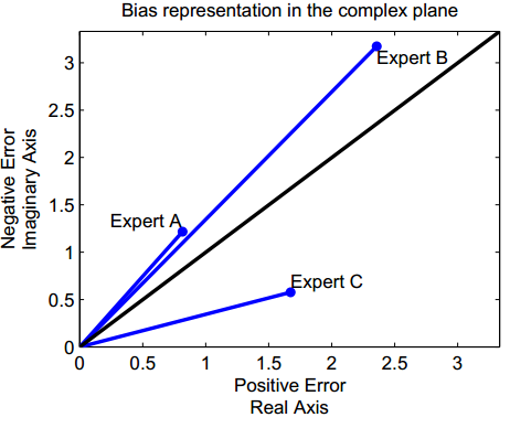
If the negative and positive errors are equal, then a and b will be equal and MRE will be on the diagonal. If the positive errors are more, or the negative, then the line will be under or over the diagonal respectively. The size of the bias is represented by how distant the MRE of each expert is from the diagonal. Also note that the MRE retains the size of errors, clearly highlighting that expert B is more inaccurate, although less biased than expert C.

Expressing the complex errors in their polar form allows us to achieve a more intuitive interpretation. Let us define γ as the angle of MRE:

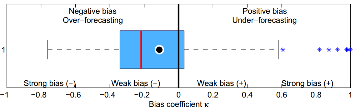
where arctan is the inverse tangent and γ is expressed in radians. If a=0 and b>0 then γ = π/2. If both a, b = 0 then γ = 0. Notice that the magnitude of MRE does not relate to the bias. Following the previous description of unbiasedness, a forecast will be unbiased for γ = π/4, while all forecast errors will have an angle γ between 0 and π/2. Instead of using γ that is expressed radians, we can define the Bias Coefficient:

The bias coefficient is a unit-free metric. A forecast that is always over the observed values will have a bias coefficient equal to -1, always over-forecasting, while the bias coefficient will be equal to 1 for the opposite case. Let us visualise the bias coefficient in the following figure. Assuming a large number of forecasts for different time series, the MRE per time series is calculated and subsequently the bias coefficient. This is then visualiased using a boxplot. The dot in the boxplot denotes the mean MRE.

The bias coefficient:

• is bounded, therefore we can characterise biases as strong or weak and have -1 and 1 as bounds of maximally biased forecasts.
• can be read similarly to the well known linear correlation coefficient. A zero value means no bias, while other values mean strong or weak bias, positive or negative. This makes it very easy to interpret and gives a non-relative understanding whether a forecast exhibits strong bias or not.
• is free of units or scale, allowing comparisons and summaries between different time series without any pre-processing.
• being unit free and bounded makes it ideal to benchmark the bias behaviour of different forecasts, methods, experts, organisations, sectors, etc.

The Root Error has several interesting properties as a metric. The bias coefficient is only one of the ways to use this new metric to characterise the performance of forecasts. This working paper introduces the Root Error and discusses many of the properties and uses of the new metric. I believe you will find it interesting.

I have updated TStools to include three new functions: mre, mre.plot and bias.coeff to help you experiment with the new metric and visualisations in the paper.

Here is a quick demonstration of how to use these functions. Let us first create some random errors:

> err <- runif(10,-10,10)

Now let us calculate the Mean Root Error of these:

> library(TStools)
> re <- mre(err)
> re
[1] 0.754675+1.924278i

Now let us calculate the bias coefficient for this:

> bias.coeff(re)
[1] -0.5241242

For the 10 random errors of this example we find a relatively strong negative bias. The bias.coeff function can also output histograms and boxplots of the bias coefficients for the input MRE.