The tsutils package for R includes functions that help with time series exploration and forecasting, that were previously included in the TStools package that is only available on github. The name change was necessary as there is another package on CRAN with the same name. The objective of TStools is to provide a development and testing ground for various functions developed by my group that has led to the creation of various packages over time, such as smooth, nnfor and now tsutils.
The package provides functions to support the following tasks:
- tests and visualisations that can help the modeller explore time series components and perform decomposition;
- modelling shortcuts, such as functions to construct lagmatrices and seasonal dummy variables of various forms;
- an implementation of the Theta method;
- tools to facilitate the design of the forecasting process, such as ABC-XYZ analyses;
- “quality of life” tools, such as treating time series for trailing and leading values.
We will look at some of these functions here, to show you how tsutils can be helpful in your forecasting projects.
Time series exploration
Exploring your time series is an important step in modelling them. Some standard questions that one has to consider is whether a time series exhibits trend and/or seasonality. First, we deal with the existence of trend. To look into this, it is useful to extranct the Centred Moving Average, and to do this you can use the functon cmav().
library(tsutils)
cma <- cmav(referrals) # referrals in a series included in the tsutils package.
The cmav() function offers a few useful arguments. By default it takes the length of the moving average from the time series information and sets it equal to its frequency. The user can override this by setting the argument ma. Another useful argument is fill=c(TRUE,FALSE) that instructs the function to fill the first and last observations of the centred moving average that are ommited in the calculation, due to the “centering”. This is done using exponential smoothing (ets() from the forecast package). This is done by default. The argument fast restricts the number of exponential smoothing models considered to speed up the calculation. Finallly the argument outplot=c(FALSE,TRUE) provides a plot of the time sereis and the calculated centred moving average. The CMA can help us identify whether there is a trend visually (see this paper for a discussion), but also to help us with statistical testing.
The function trendtest() provides a logical (TRUE/FALSE) answer for the presence of trend in a time series. It offers two alternatives, controlled by the argument type, which can take the values "aicc" or "cs" that tests by either fitting alternative exponential smoothing models and comparing their AICc or by using the Cox-Stuart test at 5% significance (you can run the test on its own using the function coxstuart()). The test can be conducted on the raw time series, or its CMA, the latter providing a cleaner signal of the low frequency components of the series, a major component of which is the trend. This is controlled by the argument extract. When this is TRUE the test is conducted on the CMA.
# Test on the CMA
trendtest(referrals, extract=TRUE)
## [1] TRUE# Test on the raw time series
trendtest(referrals, extract=FALSE)## [1] FALSEWe can see that testing on the unfiltered data provides a different response. A further (experimental) argument is mta that instructs the function to use Multiple Temporal Aggregation, as proposed in the paper that introduces MAPA. Some evidence of the effect of this is provided here, where it increases the accuracy of both approaches, AICc or Cox-Stuart testing.
The function seasplot() is handy for exploring the seasonality of the time series. This provides various arguments for controlling the result. You can manually set the seasonal length (ma – otherwise it uses frequency(y)), the starting period of the seasonal cycle (s – also picked up from the time series object, if available), assume trend being present, absent or test (trend), type of decomposition when trend is present (decomposition) and using precaclculated CMA for the decomposition (cma – use NULL for calculating internally). If there is trend in the time series (as set by the user, or tested) then the time series is first de-trended according to the decomposition setting and then the seasonal plot is produced.
There are a number of arguments to control the visualisation of seasonality. The argument outplot takes the following options:
- 0, no plot;
- 1, seasonal diagram;
- 2, seasonal boxplots;
- 3, seasonal subseries;
- 4, seasonal distribution;
- 5, seasonal density.
In addition, one can provide various arguments to the plot function (consider in the ... input), override the colouring (colour) and the labels (labels).
seasplot(referrals) ## Results of statistical testing
## Evidence of trend: TRUE (pval: 0)
## Evidence of seasonality: TRUE (pval: 0.002)
## Results of statistical testing
## Evidence of trend: TRUE (pval: 0)
## Evidence of seasonality: TRUE (pval: 0.002)The figure below exemplifies the available ploting alternatives.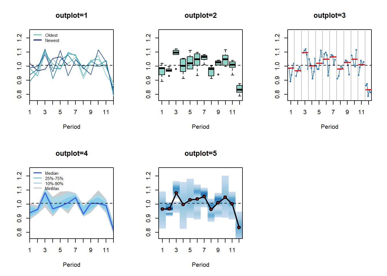 The function provides some useful results, organised in a list: the trend and seasonal compoonents, the logical result of testing for their presence and the p-value of the tests. The trend is tested using the
 coxstuart() function, while the seasonality is tested by applying the Friedman test on the data as organised for `outplot=2’, i.e. is there evidence that at least one of the ranks of the distributions of the seasonal indices is significantly different from the rest?
Finally, the function decomp() provides classical time series decomposition. Many of the arguments are similar to the seasplot function. Note that type now defines the method that is used to calculate the seasonal indices, which can be the arithmetic mean, median or a “pure seasonal” exponential smoothing model. That is, simply applying an exponential smoothing on the seasonal indices to smooth any randomness. As the later makes it complicated to extrapolate the seasonal component, the function accepts the argument h to provide predicted seasonal indices for h-steps ahead. Additionally for the calculation of the arithmetic mean one can winsorise extremes using the argument w.
dc <- decomp(referrals,outplot=TRUE)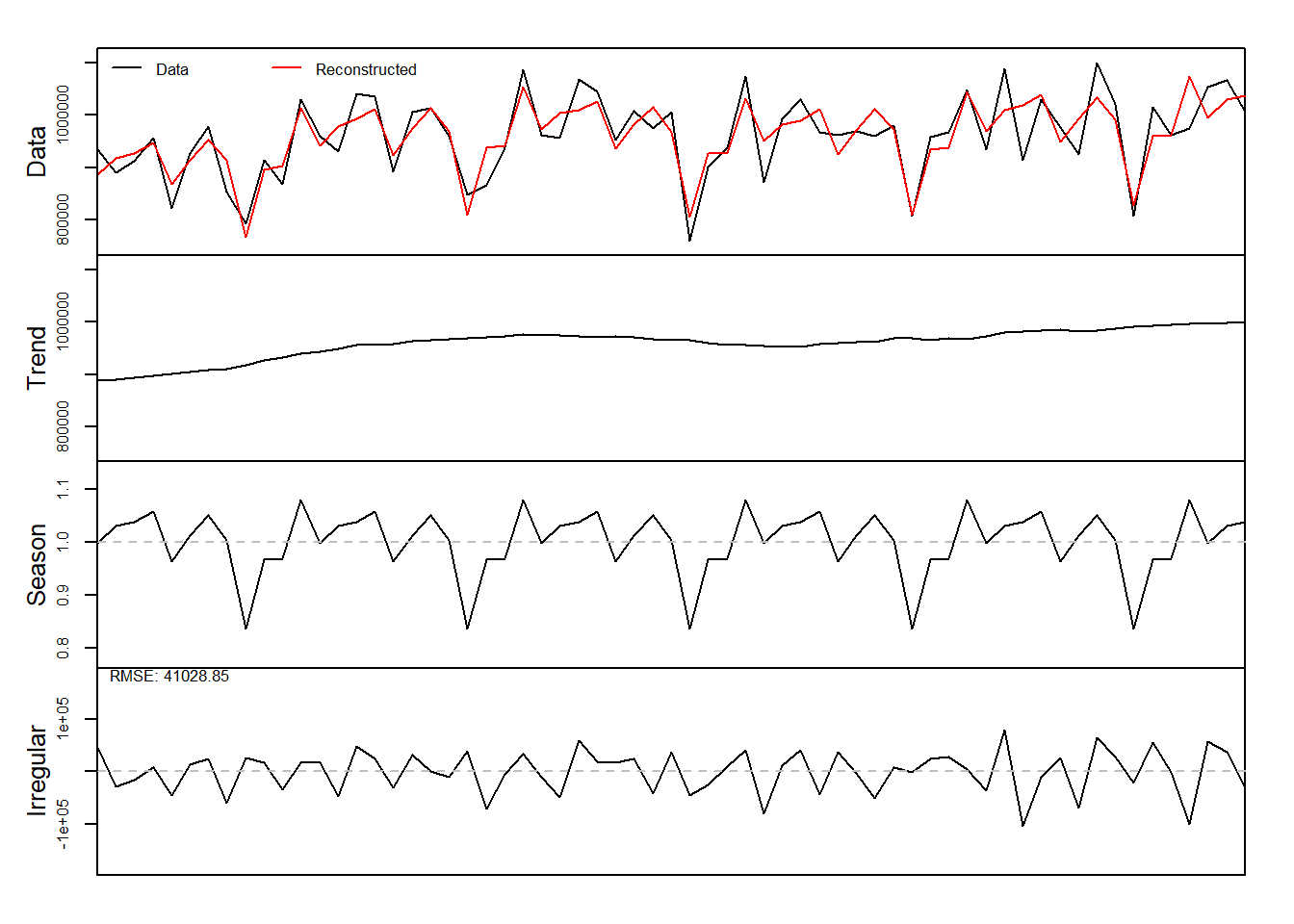
names(dc)## [1] "trend" "season" "irregular" "f.season" "g"You can see that the output of the function is a list containing the various time series components. Note that decomp() does not test for the presence of seasonality will always extract a seasonal component.
Time series modelling
There are a few fuctions that are designed with regression modelling in mind. The function lagmatrix() takes an input variable and constructs leads and lags as required.
lags <- lagmatrix(referrals, c(0,1,3:5))
head(lags,10)
## [,1] [,2] [,3] [,4] [,5]
## [1,] 933976 NA NA NA NA
## [2,] 890852 933976 NA NA NA
## [3,] 912027 890852 NA NA NA
## [4,] 955852 912027 933976 NA NA
## [5,] 821916 955852 890852 933976 NA
## [6,] 928176 821916 912027 890852 933976
## [7,] 979219 928176 955852 912027 890852
## [8,] 853812 979219 821916 955852 912027
## [9,] 792731 853812 928176 821916 955852
## [10,] 913787 792731 979219 928176 821916The first column is the original variable (lag 0), while the other columns are the requested lagged realisations. Leads are constructed by using negative numbers for the argument lag.
The function seasdummy() creates seasonal dummy variables that can be either binary or trigonometric, as defined by the argument type=c("bin","trg"). Other arguments are the number of observations to create (n), the seasonal periodicity (m), a time series (y) that is an optional argument and can be useful to get the seasonal periodicity and the starting period information. The latter is useful when the seasonality is trigonometric to get the phase of the sines and cosines correctly. Argument full retains or drops the m-th dummy variable. For linear models that would typically be set to full=FALSE. For nonlinear models this becomes a somewhat more interesting modelling question. Some evidence for neural networks is provided in this paper.
seasdummy(n=10,m=12)## [,1] [,2] [,3] [,4] [,5] [,6] [,7] [,8] [,9] [,10] [,11]
## [1,] 1 0 0 0 0 0 0 0 0 0 0
## [2,] 0 1 0 0 0 0 0 0 0 0 0
## [3,] 0 0 1 0 0 0 0 0 0 0 0
## [4,] 0 0 0 1 0 0 0 0 0 0 0
## [5,] 0 0 0 0 1 0 0 0 0 0 0
## [6,] 0 0 0 0 0 1 0 0 0 0 0
## [7,] 0 0 0 0 0 0 1 0 0 0 0
## [8,] 0 0 0 0 0 0 0 1 0 0 0
## [9,] 0 0 0 0 0 0 0 0 1 0 0
## [10,] 0 0 0 0 0 0 0 0 0 1 0For example, one can use these two functions to quick construct dynamic regression models.
Xl <- lagmatrix(referrals,c(0:2))
Xd <- seasdummy(n=length(referrals),y=referrals)
X <- as.data.frame(cbind(Xl,Xd))
colnames(X) <- c("y",paste0("lag",1:2),paste0("d",1:11))
fit <- lm(y~.,X)
summary(fit)
##
## Call:
## lm(formula = y ~ ., data = X)
##
## Residuals:
## Min 1Q Median 3Q Max
## -99439 -43116 7114 38919 98649
##
## Coefficients:
## Estimate Std. Error t value Pr(>|t|)
## (Intercept) 4.808e+05 1.695e+05 2.836 0.00672 **
## lag1 1.469e-01 1.337e-01 1.098 0.27760
## lag2 1.799e-01 1.397e-01 1.288 0.20394
## d1 1.751e+05 3.820e+04 4.584 3.38e-05 ***
## d2 1.867e+05 4.161e+04 4.488 4.64e-05 ***
## d3 2.445e+05 3.485e+04 7.015 7.75e-09 ***
## d4 1.285e+05 4.204e+04 3.056 0.00369 **
## d5 1.840e+05 3.892e+04 4.727 2.10e-05 ***
## d6 2.020e+05 3.709e+04 5.447 1.83e-06 ***
## d7 2.054e+05 3.621e+04 5.673 8.39e-07 ***
## d8 1.139e+05 3.613e+04 3.152 0.00282 **
## d9 1.698e+05 3.604e+04 4.713 2.21e-05 ***
## d10 2.168e+05 3.749e+04 5.783 5.73e-07 ***
## d11 1.616e+05 3.658e+04 4.418 5.83e-05 ***
## ---
## Signif. codes: 0 '***' 0.001 '**' 0.01 '*' 0.05 '.' 0.1 ' ' 1
##
## Residual standard error: 56250 on 47 degrees of freedom
## (2 observations deleted due to missingness)
## Multiple R-squared: 0.5882, Adjusted R-squared: 0.4743
## F-statistic: 5.165 on 13 and 47 DF, p-value: 1.365e-05Obviously, one might prefer to have the seasonal dummies as a factor variable, when these are to be coded as binary dummy variables. Users of the nnfor package may recognise these two functions. In the next release of that package, both functions will be moved to the tsutils (this is already done in the development version).
The function residout() looks at model residuals from a control chart point of view and identifies outlying ones. You can manually set the threshold over which the standardised residuals will be considered outlier (t) and whether to produce a plot (outplot).
rsd <- residout(residuals(fit))
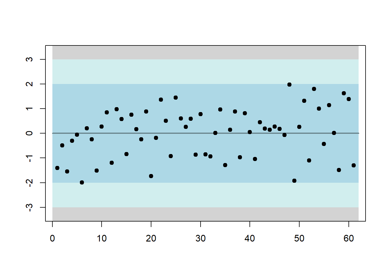
If there are outliers, their location and values are provided in the outputted list.
err <- rnorm(20)
err[5] <- err[5]+5
residout(err,outplot=FALSE)$location
## [1] 5The idea behind this function is to identify outliers so that the modeller can construct dummies to account for them or manipulate them otherwise.
A somewhat more exotic function is getOptK that provides the optimal temporal aggregation level for AR(1), MA(1) and ARMA(1,1) processes. The user defines the type of data generating process that we expect (type=c("ar","ma","arma")) and the maximum aggregation level (m). The output is the theoretically optimal aggregation level.
getOptK(referrals) # This time series is clearly not an AR(1)!## [1] 9For a discussion of the pros and cons of this theoretical calculation see this paper. My personal view is that Multiple Temporal Aggregation as implemented in MAPA or Temporal Hierarchies (thief) is a less risky modelling approach and therefore more desirable for practice.
The function theta() provides an implementation of the classical Theta method, with a few modifications. The workflow matches the one in the forecast package:
fit <- theta(referrals)
frc <- forecast.theta(fit,h=20)
plot(frc)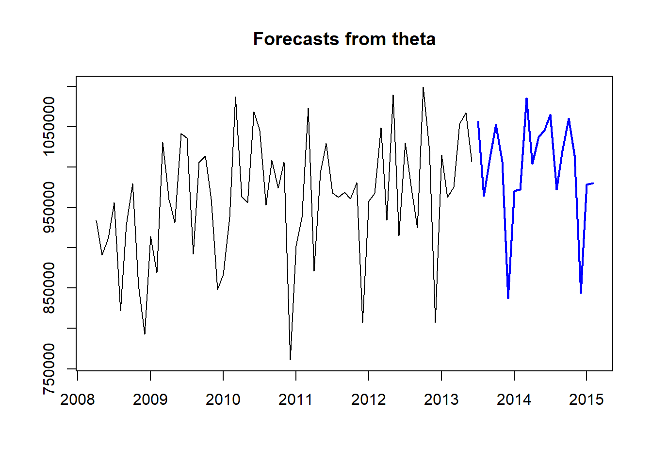 This implementation of the Theta method tests for seasonality and trend. Seasonal decomposition can be done either additively or multiplicatively and the seasonality is treated as a pure seasonal model. The various Theta components can be optimised using different cost functions. The originally proposed Theta method always assumed multiplicative seasonality and presence of trend, while all theta lines were optimised using MSE and seasonality was estimated using classical decomposition and arithmetic mean. The various arguments of the function can control how
 theta() operates: m can be used to manually set the seasonal length, sign.level the significance level for the statistical tests, cost0 to cost2 the cost function for the various components of the model, multiplicative the type of decomposition used and cma an optional pre-calculated Centred Moving Average used for decomposition and testing. Also note that since impolementation is not based on a model, it does not provide prediction intervals or information criteria.
If you are a user of thief (if not give it a try!) the function theta.thief() integrates both packages:
library(thief)
thief(referrals,forecastfunction=theta.thief)
## Jan Feb Mar Apr May Jun Jul
## 2013 1035418.8
## 2014 955320.7 957015.3 1067922.5 984519.0 1019637.9 1027866.9 1040235.2
## 2015 959464.4 961167.2 1072865.8 988823.4 1024207.9 1032495.2
## Aug Sep Oct Nov Dec
## 2013 943204.9 991756.3 1031436.6 987854.5 819194.1
## 2014 947299.6 996207.8 1036200.5 992380.8 822408.6
## 2015In this case temporal hierarchy forecasts are constructed using the Theta method, as implmemented in tsutils, at all temporal aggregation levels.
One of the major tasks in producing the appropriate forecasts for a time series is evaluating the performance of different models/methods. The nemenyi() function is helpful to perform nonparametric multiple comparisons testing. There are two considerations. First, some difference in summary performance statistics does not always mean that one forecast is indeed preferable, as differences may still be due to randomeness, and more evidence is necessary. Second, doing repeated pairwise testing between methods does not result in the desired significance in the results, as by doing this repetition is distorting your testing probabilities. The nemenyi() function first performs a Friedman test to establish that at least one method performs significantly different and then uses the post-hoc Nemenyi test to group methods by similar performance. Both tests are nonparametric, and therefore the distribution of the performance metric is not an issue.
x <- matrix( rnorm(50*4,mean=0,sd=1), 50, 4) # Generate some performance statistics
x[,2] <- x[,2]+1
x[,3] <- x[,3]+0.7
x[,4] <- x[,4]+0.5
colnames(x) <- c("Method A","Method B","Method C - long name","Method D")
nemenyi(x)
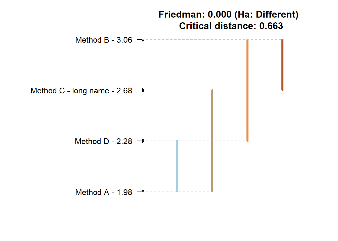
## Friedman and Nemenyi Tests
## The confidence level is 5%
## Number of observations is 50 and number of methods is 4
## Friedman test p-value: 2e-04 - Ha: Different
## Critical distance: 0.6633
The plot is fairly easy to read. Any for methods that are joined by a horizontal there is no evidence of statistically significant differences. There are multiple lines, as we can start measuring from different methods. The test is simple. For any method that is within plus/minus the critical distance (CD in the plot) from the mean rank (the values next to method names) there is no evidence of differences. The function provides different plot styles, using the argument plottype. This can be used to minic the “multiple comparison with the best” (plottype="mcb" or plottype="vmcb" for vertical alternative), the “line plot” above (plottype="line" or plottype="vline"), a detailed comparison (plottype="matrix") or output no visualisation (plottype="none").
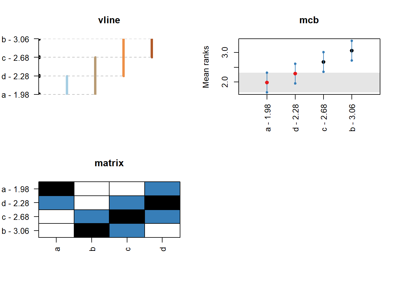
The mcb visualisation shows the performance of the various methods seperately. The dot in the middle is the mean rank of the method and the lines span te critical distance (half above and half below). For any other method that its boundaries are crossed there is no evidence of significant differences. The matrix shows on the vertical axis all methods sorted according to mean rank. On the horizontal axis they are sorted as in the input array. The balck cell is the method from which we measure and in a row (or column) any methods in blue belong to the same group of perofrmance. For example, in all the plots above, method A has no differences from d and c. Method d similarly is grouped together with a and c. When we measure from c, on the other hand, we have no evidence for significant differences from any method. When we measure from b, then both a and d have significant differences. If we are interested in the best performing group then the mcb visualisation is the simplest to consult. Otherwise matrix is the most detailed and line/vline is a compromise between the two.
Forecasting process modelling
Beyond various modelling functions, the package tsutils offers some functions for analysing the forecasting process. More specifically it helps to conduct ABC-XYZ analyses. This is done using the functions abc(), xyz() and abcxyz().
Starting with the ABC part of the analysis, given an array of time series, where each column is a time series, you can use:
x <- abs(matrix(cumsum(rnorm(5400,0,1)),36,150)) # Construct some random data
ABC <- abc(x)
print(ABC)
## ABC analysis
## Importance %
## A (20%): 39.678
## B (30%): 43.061
## C (50%): 17.261We can also plot the output, providing the concentration in each class.
plot(ABC)
Alternatively, the input can be a vector that contains the importance index for each series. The reader is referred to Ord K., Fildes R., Kourentzes N. (2017) Principles of Business Forecasting, 2e. Wessex Press Publishing Co., p.515-518 for details of how to use the ABC analysis, as well as the XYZ analysis that follows.
The user can set custom percentages for each class, or change the number of classes with the argument prc. For example:
plot(abc(x,prc=c(0.1,0.15,0.25,0.5)))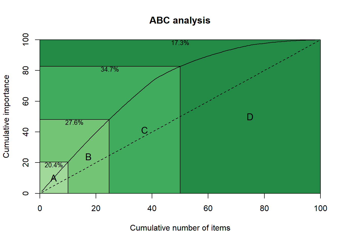
The function xyz() looks at the forecastability side. In addition to the arguments in abc() the user can select the type of forecast used to generate errors (type) and the seasonal periodicity of the series (m). For a discussion see the aforementioned reference and here. By default the naive and seasonal naive methods are used (type="naive"), but the user can opt to rely on exponential smoothing (type="ets"). The option to use the coefficient of variation is available (type="cv"), but I strongly advise against using it (see the previous references).
XYZ <- xyz(x,m=12)
plot(XYZ)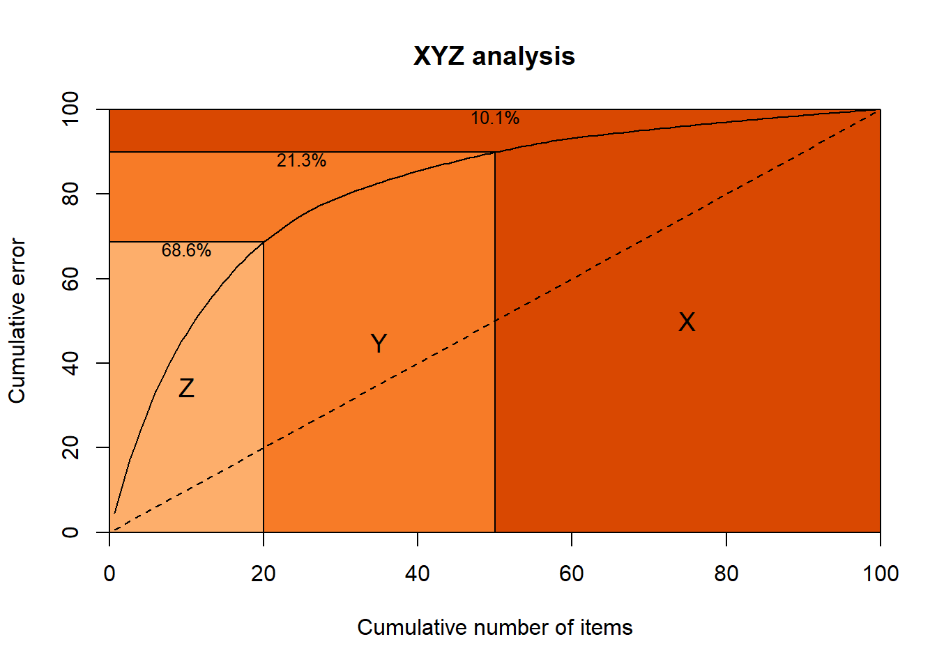
One can combine both analyses with the function abcxyz(). This can also accept a vector of forecast errors (with the argument error) that are distributed to each class of items. This vector must be equal length to the columns used to construct the ABC and XYZ analyses.
abcxyz(ABC,XYZ)
## $class
##    Z  Y  X
## A  0  0 30
## B  0  0 45
## C 30 45  0
##
## $error
## NULL
Quality of life functions
The package includes some QoL functions. The function geomean() calculates the geometric mean and accepts the same arguments as the mean().
geomean(c(0.5,1,1.5))## [1] 0.9085603mean(c(0.5,1,1.5))## [1] 1The function leadtrail() can remove leading or trailing zeros or NAs as requested. This is controlled by the argumentsrm, lead and trail.
x <- c(rep(0,2),rnorm(5),rep(0,2))
print(x)
## [1] 0.0000000 0.0000000 -0.9519769 -1.1978381 -0.9596107 -1.6142629
## [7] 0.5855328 0.0000000 0.0000000leadtrail(x)## [1] -0.9519769 -1.1978381 -0.9596107 -1.6142629 0.5855328The function wins() winsorises vectors and accepts the argument p to control how many observations are treated. If p is less than 1, then it is interpretted as a percentage. If it is bigger or equal to 1, then it is treated as number of observations.
x <- sort(round(runif(10)*10))
print(x)
## [1] 0 1 1 1 3 7 8 8 9 9wins(x,2)## [1] 1 1 1 1 3 7 8 8 8 8wins(x,0.1)## [1] 1 1 1 1 3 7 8 8 9 9There are two vectorised versions colWins() and rowWins() to speed up calculations for large arrays.
Finally, the function lambdaseq() is meant to be used with LASSO and similar. Given some response target y and regressors x it calculates a sequence of lambdas from the OLS solution to the penalty that removes all regressors from the model. If weighted LASSO will be used, then the argument weigth can beused to account for that. To switch to ridge regression or elastic nets use the argument alpha. How many lambdas are produced (nLambda) and how the lambda decreases (lambdaRatio) can be controlled. The argument standardise preprocess the variables, while the arguement addZeroLamda does as it says and adds the OLS solution lambda in the output vector.
y <- mtcars[,1]
x <- as.matrix(mtcars[,2:11])
lambda <- lambdaseq(x, y)[[1]]
plot(lambda)
This can be directly used with the glmnet package, or with custom shrinkage estimators (the motivation behind building this function!).
library(glmnet)
fit.lasso <- cv.glmnet(x, y, lambda = lambda)
Users of TStools will not find any new functionality in tsutils yet. Under the hood there are various improvements and better documentation. Where necessary, the functions point to useful references and examples. Most importantly, these functions are now in CRAN and safe to use! The plan is to keep expanding tsutils with more functions that graduate from the development TStools.
Happy forecasting!
Nikos, thank you for this post. Its very inspiring.
This is wonderful!
Your posts are really great.
Had a query regarding data transformation during time series modelling, We use different transformations such as log or box cox transformations before applying time series models.I would like to know is it fine to do scaling(multipying or dividing by a constant) on the time series before applying time series models(Models like arima, ets , stlf etc).
I do not see why scaling would affect linear models. We can always do some tricks to split the estimation. For instance in lasso regression we take away the mean and do not estimate it as part of the regression, but do it separately. You could in principle do that with ETS, Arima, etc. However, keep in mind that if you are using ETS with multiplicative specifications, you need to avoid introducing zeros and make any proportional changes (i.e. multiply/divide), as otherwise you will break the multiplicative connection between the components and the level!