Extrapolative forecasting, using models such as exponential smoothing, is arguably not very complicated from a mathematical point of view, but it requires a shift in logic in terms of what is a good forecast. For this discussion I will use a simple form of exponential smoothing to demontrate my point.
1. The forecasting model: single exponential smoothing
The forecast is calculated as:
 F_t") ,
,
where  is the forecast and
  is the actual historical value for period
  . The smoothing parameter
  is a value between 0 and 1. In its simplest interpretation this can be seen as a weighted moving average, where the distribution of weight is controlled by the smoothing parameter. Without going into too much detail we can say the following:
- A low value for
 results in a long weighted moving average and in turn in a very smooth model fit;
- A high value results in a short weighted moving average that update the forecast very fast according to the most recent actual values of the time series.
For example consider the case when  , the forecast equation becomes:
  , which is the same as the Naive method and in practice makes the forecast equal to the last observed value. No older observations are considered and no smoothing occurs. If we want to be proper with our model, then neither values of 0 or 1 are allowed for the smoothing parameter, but the above example is quite illustrative and therefore useful.
2. Forecasting sales
Now that the basics of the model are explained let us look at the following example. Let us assume we have to forecast sales of a product with two years of history and we have two alternative model fits, one with smoothing parameter equal to 0.1 and one equal to 0.9.

Fig. 1. Model fit with parameter 0.1 and 0.9.
The key question is: which of the two alternatives is the best for forecasting future sales? This is a question I get quite often by practitioners and students in various forms.
The typical answer I get from people who are not trained in forecasting/statistics is that the option with parameter 0.9 is best. It indeed seems to follow the shape of past sales quite closely and arguably if we could somehow shift it to the left by one period the fit would be fantastic. Whereas on the other hand the fit based on parameter 0.1 is a flat line that does not follow the observed historic sales.
This is a reasonable argument, but unfortunately it is wrong. In fact I mislead you so far, because in the equation for single exponential smoothing I did not include the error term and therefore we focused on comparing the actual sales and the point forecast. The point forecast is simply the most probable value in the future, but it is not the only possible one! Every forecast assumes some error, as there is always unaccounted information (what we typically call noise). We should really think every forecasted value as a distribution of values, with the most probable being the point forecast. Fig. 2 illustrates this by providing both the point forecast as well as the 80% and 90% Prediction Intervals (PI), i.e. the areas within which the future actual is expected to be with 80% and 90% confidence.

Fig. 2. A period ahead forecast with prediction intervals.
Observe that as we look for higher confidence (from 80% to 90%) the PIs become wider. That already tells you something about how much confidence we have with regards to the accuracy of the point forecast!
3. Prediction Intervals
The PIs are connected to the error variance of the forecast, which for unbiased forecasts is simply the Root Mean Squared Error (RMSE):
^2}}}")
where  is the number of errors between historical and fitted values. This is also related to why we typically optimise forecasting models on squared errors: we are trying to minimise the error variance. So the smaller the RMSE the tighter are the PIs, which if our statistics are correct implies we have more confidence in our forecast. Obviously this is connected with any decisions that we may take using these forecasts, such as inventory decisions. The PIs and the safety stock are connected. For a more in-depth and relevant discussion on the connection to safety stock, as well as the problem of biased forecasts read this.
For our example forecasts we have the following RMSE:
- Parameter 0.1: RMSE = 35.9
- Parameter 0.9: RMSE = 40.4
which already informs us that we have less certainty on the predictions that are based on the smoothing parameter 0.9 that tries to follow the pattern of sales “better”. Fig 3 illustrates this for the in-sample fit for both cases.

Fig. 3. Fit to historical sales with 80% and 90% one-step ahead prediction intervals.
There are a few things we can say about Fig. 3. First consider the plot for parameter 0.1. You can see that most historical sales are within the 90% prediction interval, as the name suggests. The 80% prediction interval does a decent job as well. On the other hand the fitted value (the point forecast) does not follow the sales pattern and if we would consider this as the only indication of a good forecast, we would reject it. Compare this with the plot for parameter 0.9. Now things are much more erratic. The prediction intervals are more risky, in the sense that more points are outside or just marginally inside, even though the intervals themselves are wider. The fitted values still do not fare better in being close to the historical sales (for each month!).
Consider another aspect of this, suppose that you need to take some decision on the forecasts. The “smooth” one based on the low parameter provides a very stable forecast and PIs. So for example running an inventory at 90% service level, more or less implies having to meet a demand & safety stock looking similar to the 90% PI. Now consider taking the same decision using the predictions based on parameter 0.9. You will need to revise the plan all the time, as the predictions and respective PIs are very volatile.
The true forecasts are even more striking, as it is shown in Fig. 4. For parameter 0.1 the prediction intervals are tighter, implying more confidence in our predictions, but also less costly decisions, such as lower safety stock. On the other hand the second forecast requires much wider prediction intervals, more uncertainty and the forecast does not look more reasonable! In both cases we get a flat line of forecasts, as this is what single exponential smoothing is capable of producing as a forecast. The impression that is was doing something more was misleading. Observe that as we are calculating the PIs for multiple steps ahead these typically become wider. Again, consider the cost implications.
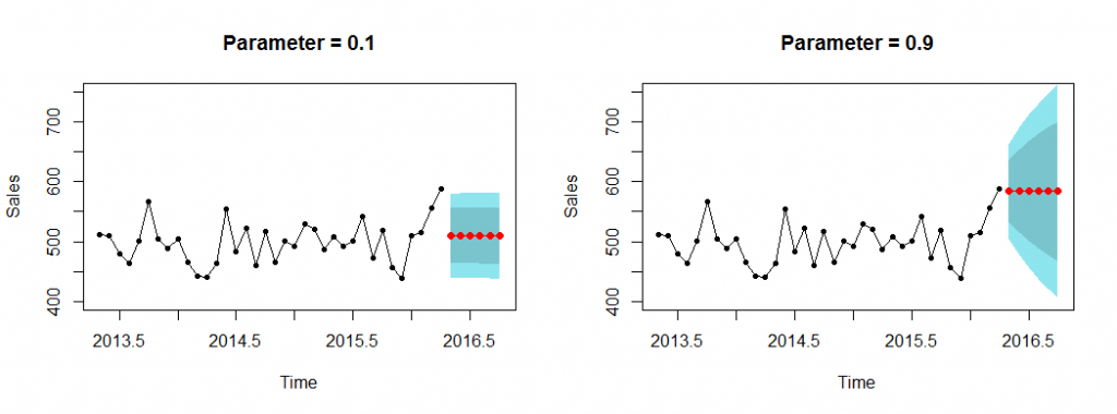
Fig. 4. Forecasts with 80% and 90% prediction intervals.
4. A fundamental idea
Real time series contain noise, which cannot be forecasted. Therefore our objective should be to capture only the underlying overall structure and not the specific patterns that are most likely due to noise. Think what your forecasting model (or method) is capable of capturing and try to do only that. Single exponential smoothing is only capable of capturing the “level” of the time series. It is incapable of capturing trend, seasonality or special events and we should not abuse the model to do so. This will only result in very uncertain predictions, with substantial cost implications that only look more “reasonable” if we consider only the point forecasts. Once the PIs are calculated it becomes clear that we are making life much harder for us.
Long story short:
- The point forecast will be (always) wrong, so instead one should look at prediction intervals.
- Consider your model and try to fit to the structure it is able to do; do not be tempted to “explain” everything with your model. The latter will make forecasts to follow around noise, resulting in poor PIs and expensive decisions.
Obviously more complex models are able to capture more patterns and details from a time series, but again that in itself may just lead to over-fitting, a topic I will not go into in this post!
I hope this illustration helps explain why we should not try to make our extrapolative forecasts match the historical patterns fully, and switch from thinking about point forecasts to distributions, as conveyed by the prediction intervals.
A final note: my intention was not to be exact with my statistics, but rather illustrate a point! There is much more to be said about PIs, parameter and model selection and so on.
You may find it helpful to experiment with different exponential smoothing models and parameters and PIs using this interactive demo.


