In most business forecasting applications, the problem usually directs the sampling frequency of the data that we collect and use for forecasting. Conventional approaches try to extract information from the historical observations to build a forecasting model. In this article, we explore how transforming the data through temporal aggregation allows us to gather additional information about the series at hand, resulting in better forecasts. We discuss a newly introduced modelling approach that combines information from many different levels of temporal aggregation, augmenting various features of the series in the process, into a robust and accurate forecast.
- Temporal aggregation can aid the identification of series characteristics, as these are enhanced across different frequencies. Moreover, this simple trick reduces intermittency, allowing the use of established conventional forecasting methods for slow moving data.
- Using multiple temporal aggregation levels can lead to substantial improvements in terms of forecasting performance, especially for longer horizons, as the various long term components of the series are better captured.
- Combining across different levels of aggregation leads to estimates that are reconciled across all frequencies. From a practitioner’s point of view, this is very important, as it produces forecasts that are reconciled for operational, tactical and strategic horizons.
- The associated R package MAPA allows for direct use of this algorithm in practice through the open source R statistical software.
Why temporal aggregation?
Typically, for short-term operational forecasts monthly, weekly, or even daily data are used. On the other hand, a common suggestion is to use quarterly and yearly data to produce long-term forecasts. This type of data does not contain the same amount of details and often are smoother, providing a better view of the long term behaviour of the series. Of course, forecasts produced from different frequencies of the series are bound to be different, often making the cumulative operational forecasts over a period different than the tactical or strategic forecasts derived from the cumulative demand for the same period. Nonetheless, in practice, it is most common that the same data and models will be used to produce both short and long term forecasts, with apparent limitations, in particular for the long-horizon forecasts.
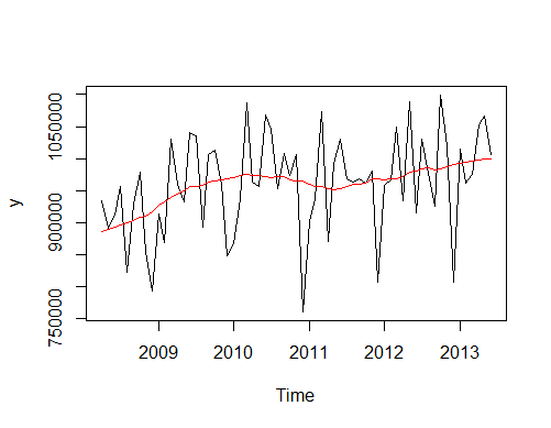
Different frequencies of the data can reveal or conceal the various time series features. When fast moving time series are considered, random variations and seasonal patterns are more apparent in daily, weekly or monthly data. Using non-overlapping temporal aggregation it is easy to construct lower frequency time series. The level of aggregation refers to the size of the time buckets in the temporal aggregation procedure and is directly linked with the frequency of the data. The increase of the aggregation level results in a series of lower frequency. At the same time, this process acts as a filter, smoothing the high frequency features and providing a better approximation of the long-term components of the data, such as level, trend and cycle. Notice in Fig. 1 how the series changes for various levels of aggregation. The original monthly series is dominated by the seasonal component, while at the 12th level of aggregation, the now annual series, is dominated by a shift in the level and a weak trend.

Fig. 1. A monthly fast-moving time series at different levels of non-overlapping temporal aggregation.
In the case of intermittent demand data, moving from higher (monthly) to lower (yearly) frequency data reduces (or even removes) the intermittence of the data, minimising the number of periods with zero demands. This can make conventional forecasting methods applicable to the problem. Fig. 2 demonstrates how such time series change behaviour as the level of the aggregation changes.

Fig. 2. A monthly slow-moving time series at different levels of non-overlapping temporal aggregation.
The presence and the magnitude of such time series features, both for fast- and slow-moving items, affects forecasting accuracy. So, the obvious question for a practising forecaster is: “Which aggregation level of my data should I use?”
Don’t trust your models!
As the time series features change with the frequency of the data (or the level of aggregation), different methods will be identified as optimal. These will produce different forecasts, which will ultimately lead to different decisions. In essence, we have to deal with the true model uncertainty, that is the appropriateness or misspecification of the model identified as optimal at a specific level of data aggregation. Even if we ignore the issue of temporal aggregation, with a simple time series we have two major types of uncertainties: i) data uncertainty: are we just very lucky, or unlucky with the sample we have? as more observations become available how would our model and its parameters change? and ii) model uncertainty: is the model or its parameters appropriate, or because of potential optimisation issues the model provides poor forecasts? The second problem is exacerbated for models with many degrees of freedom. Temporal aggregation reveals these differences and forces us to face this issue.
A potential answer to this issue is to try to consider all alternative view of your data, by using multiple aggregation levels, therefore reducing the aforementioned uncertainties. Then model each one separately, capturing best the different time series features that are amplified at each level. As the models will be different, instead of preferring a single one, combine them (or their forecasts) into a robust final forecast that takes into account information from all frequencies of the data.
So, what we propose is not to trust a single model on a single aggregation level of the data, which will avoidably lead to the selection of a single “optimal” model. Instead, consider multiple aggregation levels. This approach attempts to reduce the risk of selecting a bad model, parameterised on a single view of data, thus it mitigates the importance of model selection.
The how-to
In this section we explain how the proposed Multiple Aggregation Prediction Algorithm (MAPA) should be applied in practice, through three steps: aggregation, forecast and combination. A graphical illustration of the proposed framework is presented in Fig. 3, contrasting it with the standard forecasting approach that is usually applied in practice.

Fig. 3. The standard versus the MAPA forecasting approach.
Step 1: Aggregation.
In the standard approach the input of the statistical forecast methods is a single frequency of the data, usually the sampling that has been used during the data collection process or the one where forecasts will be used later on. So, the aggregation level is driven either from data availability or intended use of the forecasts. On the other hand, the MAPA uses multiple instances of the same data, which correspond to the different frequencies or aggregation levels. Suppose we have 4 years of monthly observations (48 data points). In order to transform these to quarterly data (1 quarter=3 months), we define 48/3 = 16 time-buckets. Then, we aggregate, using simple summation, as to calculate the cumulative demand over each of these time-buckets. This process will create 16 aggregated observations that will match the required quarterly frequency. In this case, the aggregation level is equal to 3 periods, while the transformed frequency is equal to 1/3 of the original.
In the case that the selected aggregation level is not a multiplier of the available observations at the original frequency, then some data points may be dropped out through this temporal aggregation process. Continuing our previous example, if the aggregation level is set to 5, then only 9 time buckets can be defined, corresponding to 45 monthly observations. In this case, 3 monthly periods are discarded. We choose to discard observations from the beginning of the series, as the latter ones are considered as more relevant.
This process of transforming the original data to alternative (lower) frequencies, using multiple aggregation levels, can continue as long as all transformed series have enough data to produce statistical forecasts. If the original sampling frequency is monthly data, and given that companies usually hold 3 to 5 years of history, we suggest that the aggregation process continues up to the yearly frequency (aggregation level equal to 12 periods). This will also be adequate to highlight long-term movements of the series.
In any case, while the starting frequency is always bounded from the sampling of the raw data, we propose that the upper level of aggregation should reach at least the annual level, where seasonality is filtered completely from the data and long-term (low frequency) components, such as trend, dominate. Of course, the range of aggregation levels should contain the ones that are relevant to the intended use of the forecasts: for example monthly forecasts for S&OP, or yearly forecasts for long-term planning. This ensures that the resulting MAPA forecast captures all relevant time series features and therefore provides temporally reconciled forecasts.
The output of this first step is a set of series, all corresponding to the same base data but translated to different frequencies.
Step 2: Forecasting.
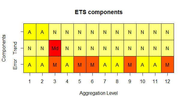
Each one of the series calculated in step 1 should be forecasted separately. In the forecasting literature, several automatic model selection protocols exist. For fast-moving items exponential smoothing is regarded as reliable and relatively accurate. It corresponds to models that may include trend (damped or not) and seasonality, while allowing for multiple forms of interaction (additive or multiplicative). A widely used approach is the automatic selection of the best model form, based on the minimisation of a predefined information criterion (such as the AIC). It is expected that on our set of series different models will be selected across the various aggregation levels. Seasonality and various high frequency components are expected to be modelled better at lower aggregation levels (such as monthly data), while the long-term trend will be better captured as the frequency is decreased (yearly data).
In the case of intermittent demand series, there are classification schemes that allow selecting between the two most widely used forecasting methods: Croston’s method and the Syntetos-Boylan Approximation (SBA). Under such schemes, the levels of intermittency and the variability of the demand distinguish which method is more appropriate. Using multiple aggregation levels will change both the intermittence and the variability, so we expect that different methods will be identified as optimal across all frequencies. Furthermore, at higher levels of aggregation the resulting series may contain no zero demand periods. In these cases, we propose using conventionally optimised Simple Exponential Smoothing, taking advantage of its good performance in non-intermittent time series. Moreover, it might be the case that the transformation of the data from slow-moving to fast-moving may reveal regular time series components (such as trend or seasonality) that may not exist at the lower levels of granularity where noise is the dominant component. Any time series at a sufficiently high frequency of sampling is intermittent, therefore these cases should be considered as a continuum.
The output of this step is multiple sets of forecasts, each one corresponding to an alternative frequency.
Step 3: Combination.
The final stage of the proposed MAPA approach refers to the appropriate combination of the different forecasts derived from the alternative frequencies.
Before being able to combine the forecasts produced from the various frequencies, we need to transform them back to the original frequency. While the aggregation of forecasts from lower aggregation levels is straightforward, disaggregation can be more complicated. Many alternative strategies have been discussed in the literature, however simply dividing an observation into equal parts at the higher frequency level has been shown to be very effective and simple to use. Consider, for example, that after the forecasting step we have some aggregated forecasts at the quarterly frequency. In order to transform each one of these point forecasts to the original (monthly) frequency, we simply divide them by three and use the same value for all three months. So, the forecast for January will be the same as the forecast of February or March, and all these will be equal to the forecast of Q1 divided by 3.
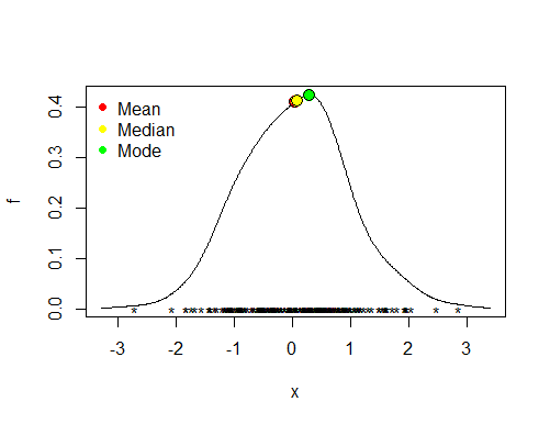
Once all forecasts from the various aggregation levels are translated back to the original frequency, these are subsequently combined into a final forecast. The combination can be done by calculating averages, medians or using other operators, such as trimmed means of the forecasts. We have found that both means and medians performed well, although the latter are more appropriate to ensure that the combined final forecasts are not affected from extreme values.
It may be the case that the indented use of the forecasts is at a different frequency from the data sampling one. Or it might be that forecasts from various aggregation levels are needed for operational, tactical or strategic planning. To achieve this, simply aggregate the final forecast to the desired level(s). A convenient property of MAPA forecasts is that they are appropriate for all these levels, as they contain information from all. Therefore such forecasts on various aggregation levels are temporally reconciled and there is no longer a need to work out how to ensure that these forecasts agree, which otherwise would typically be different.
The case of seasonality
One problem that arises from the application of the algorithm described above is with regard to the extreme dampening of the seasonal component of the time series. Consider the case of monthly data that are converted to all frequencies down to yearly. If the original series is seasonal, then seasonality will be modelled only on the aggregation levels 1 (which corresponds to the original frequency), 2, 3, 4 and 6. At the same time, seasonality will not be modelled at any of the other aggregation levels considered, either being fractional or completely filtered-out.
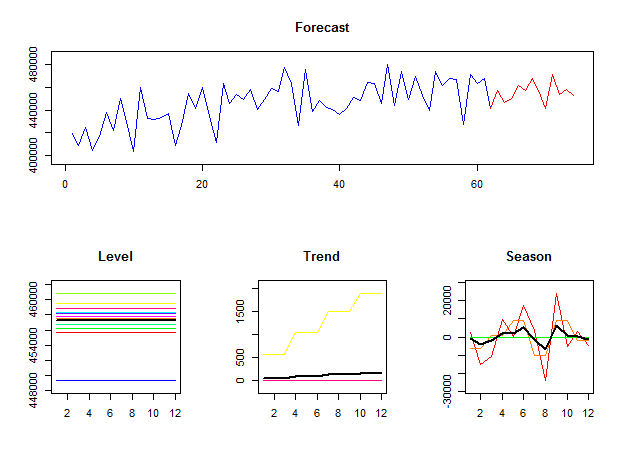
Calculating the simple combination across the forecasts of all levels will essentially dampen the seasonal pattern. This is illustrated in Fig. 4, where the models, one with seasonality (red) and one without (green) are combined and the resulting forecast has a poor fit, due to the dampening of the seasonality.

Fig. 4. Example of dampened seasonal component due to forecast combination.
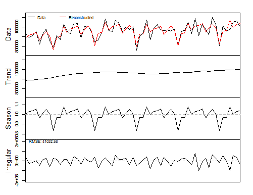
In order to address this issue the combination should be done at model components and not the forecasts. This is trivial when using the exponential smoothing family of methods, as it provides estimates for each component (level, trend, and seasonality) separately. The combination of the seasonal component will only take into account the aggregation levels where seasonality is permitted (1, 2, 3, 4 and 6). On the other hand, level and trend will be modelled at each level. If at one level a model with no trend is selected, then the trend component for that aggregation level is equal to zero. Therefore instead of combining the forecasts, one has to first combine all the level estimates from the various aggregation levels, then all the trend estimates and then the seasonal estimates. The resulting combined components are then used to calculate the final forecast, in the same way as one would do with conventional exponential smoothing.
Other ways of tackling this modelling issue would include the consideration of only some of the aggregation levels or the introduction of models that can deal with fractional seasonality.
Does it worth the extra effort?
The short answer is yes! The MAPA approach has been tested on both fast-moving and slow-moving demand data, providing improved forecasting performance when compared with traditional approaches. In more detail, the proposed approach gives better estimates both in terms of accuracy and bias. In the case of fast-moving data, the MAPA improves on exponential smoothing at most data frequencies, while being especially accurate at longer-term forecasts. This is a direct outcome of fitting models at high aggregation levels, where the level and the long-term trend of the series are best identified. In the case of slow-moving data, the MAPA, under the enhanced selection scheme (Croston-SBA-SES), performs better when compared to any single method, while its performance is also superior to that of the original selection scheme (Croston-SBA).
On top of any improvements on the forecasting performance of the MAPA, another advantage of this algorithm is that the decision maker does not have to a-priori select a single aggregation level. While, in some cases, setting the aggregation level to be equal with the lead time plus the review period makes sense, removing this hyper-parameter can be regarded as an advantage, simplifying the forecasting process.
It’s not only about accuracy
Although there are accuracy and robustness benefits from using MAPA, the key advantage is an organisational one. Combining multiple temporal aggregation levels (thus capturing both high and low frequency components) leads to more accurate forecasts for both short and (especially) long horizons. Most importantly, this strategy provides reconciled forecasts across all frequencies, which is suitable for aligning operational, tactical and strategic decision making. This is useful for practice as the same forecast can be used for all three levels of planning.
Therefore, forecasts and decisions are reconciled and there is no need to alter or prefer forecasts from a particular level, something that in practice is often done ad-hoc with detrimental effects. This is a significant drive towards the “one-number” forecast, where several decisions and organisational functions are based on the same view about the future, thus aligning them. It is not uncommon in practice that short term operational forecasts, driving demand planning and inventory management are incompatible with long-term budget forecasts. MAPA addresses this issue by providing a single reconciled view across the various planning horizons. This is just the first step towards the fully reconciled forecasts within an industrial setting. Cross-sectional reconciliation and effective interaction and communication of the different stakeholders are only some of the remaining aspects of the same problem.
Use it in practice
If you are interested in using this approach for forecasting a starting point is the MAPA package for R. Follow that link for examples on how to run MAPA with your own data.
Further reading
N. Kourentzes, F. Petropoulos and J. R. Trapero, 2014, Improving forecasting by estimating time series structural components across multiple frequencies. International Journal of Forecasting, 30: 291-302.
F. Petropoulos and N. Kourentzes, 2014, Forecast combinations for intermittent demand. Journal of Operational Research Society.
This text is an adapted version of:
F. Petropoulos and N. Kourentzes, 2014, Improving Forecasting via Multiple Temporal Aggregation, Foresight: The International Journal of Applied Forecasting.


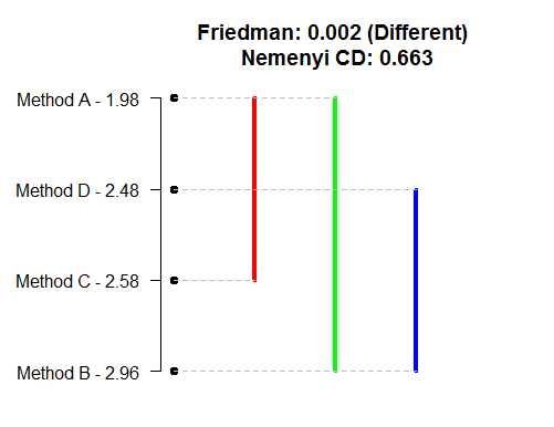
}{6N}}") ,
, is the confidence level,
  is the number of models and
  is the number of measurements. To calculate
  the Studentised range statistic for infinite degrees of freedom divided by
  is used. The values of
  can be download