Forecasting with MLPs
With the nnfor package you can either produce extrapolative (univariate) forecast, or include explanatory variables as well.
Univariate forecasting
The main function is mlp(), and at its simplest form you only need to input a time series to be modelled.
library(nnfor)
fit1 <- mlp(AirPassengers)
print(fit1)
## MLP fit with 5 hidden nodes and 20 repetitions.
## Series modelled in differences: D1.
## Univariate lags: (1,2,3,4,5,6,7,8,10,12)
## Deterministic seasonal dummies included.
## Forecast combined using the median operator.
## MSE: 7.4939.The output indicates that the resulting network has 5 hidden nodes, it was trained 20 times and the different forecasts were combined using the median operator. The mlp() function automatically generates ensembles of networks, the training of which starts with different random initial weights. Furthermore, it provides the inputs that were included in the network. This paper discusses the performance of different combination operators and finds that the median performs very well, the mode can achieve the best performance but needs somewhat larger ensembles and the arithmetic mean is probably best avoided! Another interesting finding in that paper is that bagging (i.e. training the network on bootstrapped series) or using multiple random training initialisations results in similar performance, and therefore it appears that for time series forecasting we can avoid the bootstrapping step, greatly simplifying the process. These findings are embedded in the default settings of nnfor.
You can get a visual summary by using the plot() function.
plot(fit1)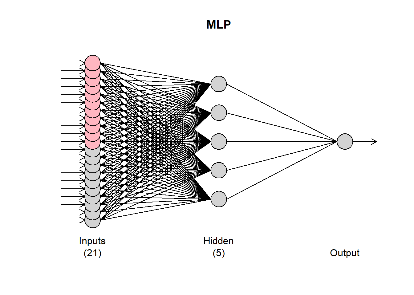
The grey input nodes are autoregressions, while the magenta ones are deterministic inputs (seasonality in this case). If any other regressors were included, they would be shown in light blue.
The mlp() function accepts several arguments to fine-tune the resulting network. The hd argument defines a fixed number of hidden nodes. If it is a single number, then the neurons are arranged in a single hidden node. If it is a vector, then these are arranged in multiple layers.
fit2 <- mlp(AirPassengers, hd = c(10,5))
plot(fit2)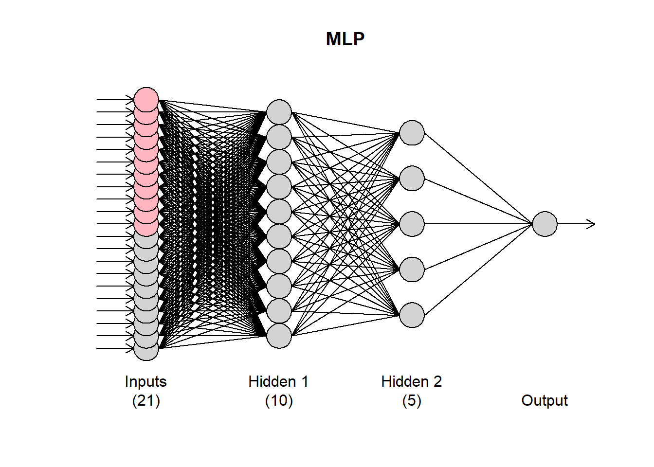
We will see later on how to automatically select the number of nodes. In my experience (and evidence from the literature), conventional neural networks, forecasting single time series, do not benefit from multiple hidden layers. The forecasting problem is typically just not that complex!
The argument reps defines how many training repetitions are used. If you want to train a single network you can use reps=1, although there is overwhelming evidence that there is no benefit in doing so. The default reps=20 is a compromise between training speed and performance, but the more repetitions you can afford the better. They help not only in the performance of the model, but also in the stability of the results, when the network is retrained. How the different training repetitions are combined is controlled by the argument comb that accepts the options median, mean, and mode. The mean and median are apparent. The mode is calculated using the maximum of a kernel density estimate of the forecasts for each time period. This is detailed in the aforementioned paper and exemplified here.
The argument lags allows you to select the autoregressive lags considered by the network. If this is not provided then the network uses lag 1 to lag m, the seasonal period of the series. These are suggested lags and they may not stay in the final networks. You can force that using the argument keep, or turn off the automatic input selection altogether using the argument sel.lag=FALSE. Observe the differences in the following calls of mlp().
mlp(AirPassengers, lags=1:24)## MLP fit with 5 hidden nodes and 20 repetitions.
## Series modelled in differences: D1.
## Univariate lags: (1,2,4,7,8,9,10,11,12,13,18,21,23,24)
## Deterministic seasonal dummies included.
## Forecast combined using the median operator.
## MSE: 5.6388.mlp(AirPassengers, lags=1:24, keep=c(rep(TRUE,12), rep(FALSE,12)))## MLP fit with 5 hidden nodes and 20 repetitions.
## Series modelled in differences: D1.
## Univariate lags: (1,2,3,4,5,6,7,8,9,10,11,12,13,18,21,23,24)
## Deterministic seasonal dummies included.
## Forecast combined using the median operator.
## MSE: 3.6993.mlp(AirPassengers, lags=1:24, sel.lag=FALSE)## MLP fit with 5 hidden nodes and 20 repetitions.
## Series modelled in differences: D1.
## Univariate lags: (1,2,3,4,5,6,7,8,9,10,11,12,13,14,15,16,17,18,19,20,21,22,23,24)
## Deterministic seasonal dummies included.
## Forecast combined using the median operator.
## MSE: 1.7347.In the first case lags (1,2,4,7,8,9,10,11,12,13,18,21,23,24) are retained. In the second case all 1-12 are kept and the rest 13-24 are tested for inclusion. Note that the argument keep must be a logical with equal length to the input used in lags. In the last case, all lags are retained. The selection of the lags heavily relies on this and this papers, with evidence of its performance on high-frequency time series outlined here. An overview is provided in: Ord K., Fildes R., Kourentzes N. (2017) Principles of Business Forecasting 2e. Wessex Press Publishing Co., Chapter 10.
Note that if the selection algorithm decides that nothing should stay in the network, it will include lag 1 always and you will get a warning message: No inputs left in the network after pre-selection, forcing AR(1).
Neural networks are not great in modelling trends. You can find the arguments for this here. Therefore it is useful to remove the trend from a time series prior to modelling it. This is handled by the argument difforder. If difforder=0 no differencing is performed. For diff=1, level differences are performed. Similarly, if difforder=12 then 12th order differences are performed. If the time series is seasonal with seasonal period 12, this would then be seasonal differences. You can do both with difforder=c(1,12) or any other set of difference orders. If difforder=NULL then the code decides automatically. If there is a trend, first differences are used. The series is also tested for seasonality. If there is, then the Canova-Hansen test is used to identify whether this is deterministic or stochastic. If it is the latter, then seasonal differences are added as well.
Deterministic seasonality is better modelled using seasonal dummy variables. by default the inclusion of dummies is tested. This can be controlled by using the logical argument allow.det.season. The deterministic seasonality can be either a set of binary dummies, or a pair of sine-cosine (argument det.type), as outlined here. If the seasonal period is more than 12, then the trigonometric representation is recommended for parsimony.
The logical argument outplot provides a plot of the fit of network.
The number of hidden nodes can be either preset, using the argument hd or automatically specified, as defined with the argument hd.auto.type. By default this is hd.auto.type="set" and uses the input provided in hd (default is 5). You can set this to hd.auto.type="valid" to test using a validation sample (20% of the time series), or hd.auto.type="cv" to use 5-fold cross-validation. The number of hidden nodes to evaluate is set by the argument hd.max.
fit3 <- mlp(AirPassengers, hd.auto.type="valid",hd.max=8)
print(fit3)
## MLP fit with 4 hidden nodes and 20 repetitions.
## Series modelled in differences: D1.
## Univariate lags: (1,2,3,4,5,6,7,8,10,12)
## Deterministic seasonal dummies included.
## Forecast combined using the median operator.
## MSE: 14.2508.Given that training networks can be a time consuming business, you can reuse an already specified/trained network. In the following example, we reuse fit1 to a new time series.
x <- ts(sin(1:120*2*pi/12),frequency=12)
mlp(x, model=fit1)
## MLP fit with 5 hidden nodes and 20 repetitions.
## Series modelled in differences: D1.
## Univariate lags: (1,2,3,4,5,6,7,8,10,12)
## Deterministic seasonal dummies included.
## Forecast combined using the median operator.
## MSE: 0.0688.This retains both the specification and the training from fit1. If you want to use only the specification, but retrain the network, then use the argument retrain=TRUE.
mlp(x, model=fit1, retrain=TRUE)## MLP fit with 5 hidden nodes and 20 repetitions.
## Series modelled in differences: D1.
## Univariate lags: (1,2,3,4,5,6,7,8,10,12)
## Deterministic seasonal dummies included.
## Forecast combined using the median operator.
## MSE: 0.Observe the difference in the in-sample MSE between the two settings.
Finally, you can pass arguments directly to the neuralnet() function that is used to train the networks by using the ellipsis ....
To produce forecasts, we use the function forecast(), which requires a trained network object and the forecast horizon h.
frc <- forecast(fit1,h=12)
print(frc)
## Jan Feb Mar Apr May
## 1961 447.3392668 421.2532515 497.5052166 521.1640683 537.4031708
## Jun Jul Aug Sep Oct
## 1961 619.5015908 707.8790407 681.0523280 602.8467629 529.0477736
## Nov Dec
## 1961 470.8292734 517.6762262plot(frc)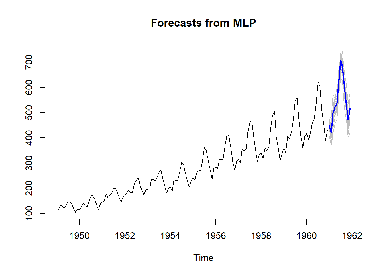
The plot of the forecasts provides in grey the forecasts of all the ensemble members. The output of forecast() is of class forecast and those familiar with the forecast package will find familiar elements there. To access the point forecasts use frc$mean. The frc$all.mean contains the forecasts of the individual ensemble members.
Using regressors
There are three arguments in the mlp() function that enable to use explanatory variables: xreg, xreg.lags and xreg.keep. The first is used to input additional regressors. These must be organised as an array and be at least as long as the in-sample time series, although it can be longer. I find it helpful to always provide length(y)+h. Let us suppose that we want to use a deterministic trend to forecast the time series. First, we construct the input and then model the series.
z <- 1:(length(AirPassengers)+24) # I add 24 extra observations for the forecasts
z <- cbind(z) # Convert it into a column-array
fit4 <- mlp(AirPassengers,xreg=z,xreg.lags=list(0),xreg.keep=list(TRUE),
            # Add a lag0 regressor and force it to stay in the model
            difforder=0) # Do not let mlp() to remove the stochastic trend
print(fit4)
## MLP fit with 5 hidden nodes and 20 repetitions.
## Univariate lags: (1,4,5,8,9,10,11,12)
## 1 regressor included.
## - Regressor 1 lags: (0)
## Deterministic seasonal dummies included.
## Forecast combined using the median operator.
## MSE: 32.4993.The output reflects the inclusion of the regressor. This is reflected in the plot of the network with a light blue input.
plot(fit4)
Observe that z is organised as an array. If this is a vector you will get an error. To include more lags, we expand the xreg.lags:
mlp(AirPassengers,difforder=0,xreg=z,xreg.lags=list(1:12))## MLP fit with 5 hidden nodes and 20 repetitions.
## Univariate lags: (1,4,5,8,9,10,11,12)
## Deterministic seasonal dummies included.
## Forecast combined using the median operator.
## MSE: 48.8853.Observe that nothing was included in the network. We use the xreg.keep to force these in.
mlp(AirPassengers,difforder=0,xreg=z,xreg.lags=list(1:12),xreg.keep=list(c(rep(TRUE,3),rep(FALSE,9))))## MLP fit with 5 hidden nodes and 20 repetitions.
## Univariate lags: (1,4,5,8,9,10,11,12)
## 1 regressor included.
## - Regressor 1 lags: (1,2,3)
## Deterministic seasonal dummies included.
## Forecast combined using the median operator.
## MSE: 32.8439.Clearly, the network does not like the deterministic trend! It only retains it, if we force it. Observe that both xreg.lags and xreg.keep are lists. Where each list element corresponds to a column in xreg. As an example, we will encode extreme residuals of fit1 as a single input (see this paper for a discussion on how networks can code multiple binary dummies in a single one). For this I will use the function residout() from the tsutils package.
if (!require("tsutils")){install.packages("tsutils")}
library(tsutils)
loc <- residout(AirPassengers - fit1$fitted, outplot=FALSE)$location
zz <- cbind(z, 0)
zz[loc,2] <- 1
fit5 <- mlp(AirPassengers,xreg=zz, xreg.lags=list(c(0:6),0),xreg.keep=list(rep(FALSE,7),TRUE))
print(fit5)
## MLP fit with 5 hidden nodes and 20 repetitions.
## Series modelled in differences: D1.
## Univariate lags: (1,2,3,4,5,6,7,8,10,12)
## 1 regressor included.
## - Regressor 1 lags: (0)
## Deterministic seasonal dummies included.
## Forecast combined using the median operator.
## MSE: 7.2178.Obviously, you can include as many regressors as you want.
To produce forecasts, we use the forecast() function, but now use the xreg input. The way to make this work is to input the regressors starting from the same observation that was used during the training of the network, expanded as need to cover the forecast horizon. You do not need to eliminate unused regressors. The network will take care of this.
frc.reg <- forecast(fit5,xreg=zz)Forecasting with ELMs
To use Extreme Learning Machines (EMLs) you can use the function elm(). Many of the inputs are identical to mlp(). By default ELMs start with a very large hidden layer (100 nodes) that is pruned as needed.
fit6 <- elm(AirPassengers)
print(fit6)
## ELM fit with 100 hidden nodes and 20 repetitions.
## Series modelled in differences: D1.
## Univariate lags: (1,2,3,4,5,6,7,8,10,12)
## Deterministic seasonal dummies included.
## Forecast combined using the median operator.
## Output weight estimation using: lasso.
## MSE: 91.288.plot(fit6)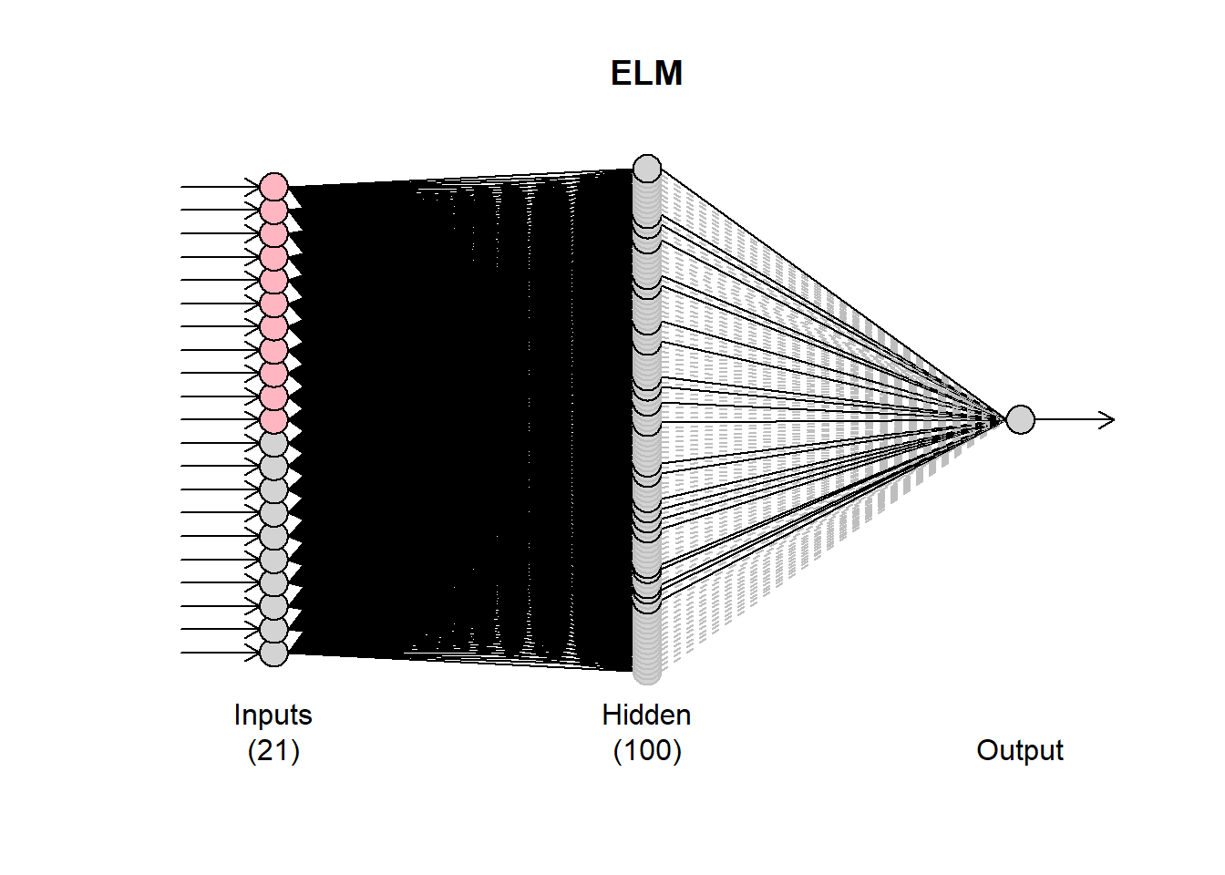
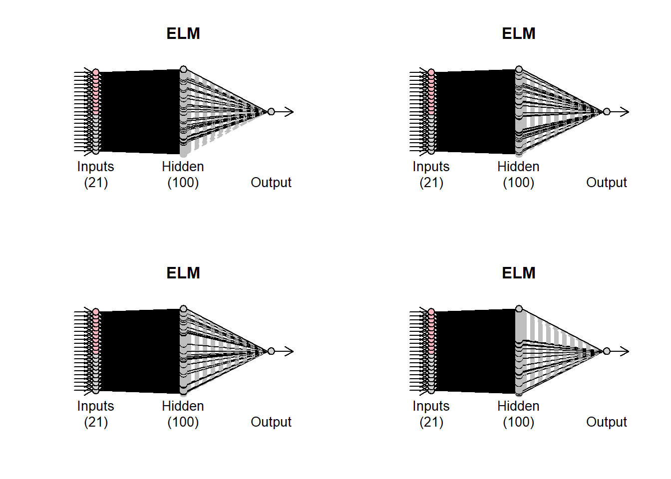
Observe that the plot of the network has some black and some grey lines. The latter are pruned. There are 20 networks fitted (controlled by the argument reps). Each network may have different final connections. You can inspect these by using plot(fit6,1), where the second argument defines which network to plot.
par(mfrow=c(2,2))
for (i in 1:4){plot(fit6,i)}
par(mfrow=c(1,1))
How the pruning is done is controlled by the argument.type The default option is to use LASSO regression (type=“lasso”). Alternatively, use can use “ridge” for ridge regression, “step” for stepwise OLS and “lm” to get the OLS solution with no pruning.
The other difference from the mlp() function is the barebone argument. When this is FALSE, then the ELMs are built based on the neuralnet package. If this is set to TRUE then a different internal implementation is used, which is helpful to speed up calculations when the number of inputs is substantial.
To forecast, use the forecast() function in the same way as before.
forecast(fit6,h=12)## Jan Feb Mar Apr May
## 1961 449.0982276 423.0329121 455.7643540 488.5096713 499.3616506
## Jun Jul Aug Sep Oct
## 1961 567.7486203 645.6309202 622.8311280 543.9549163 495.8305278
## Nov Dec
## 1961 429.9258197 468.7921570Temporal hierarchies and nnfor
People who have followed my research will be familiar with Temporal Hierarchies that are implemented in the package thief. You can use both mlp() and elm() with thief() by using the functions mlp.thief() and elm.thief().
if (!require("thief")){install.packages("thief")}
library(thief)
thiefMLP <- thief(AirPassengers,forecastfunction=mlp.thief)
# Similarly elm.thief:
thiefELM <- thief(AirPassengers,forecastfunction=elm.thief)
par(mfrow=c(1,2))
plot(thiefMLP)
plot(thiefELM)
par(mfrow=c(1,1))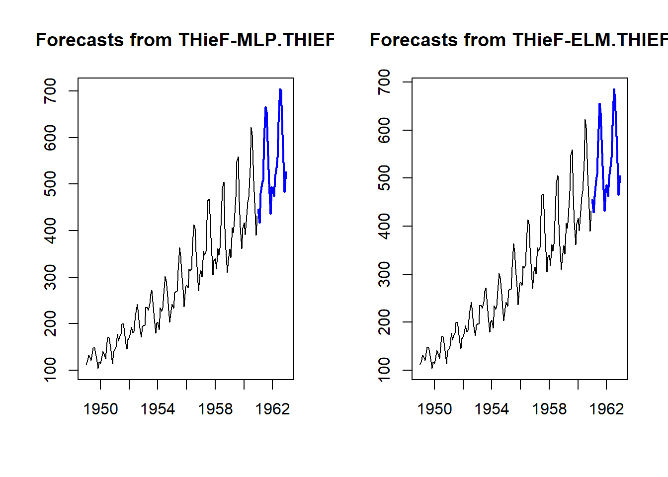
This should get you going with time series forecasting with neural networks.
Happy forecasting!


 (1)
(1) is the forecast for period t+h, constructed at period t (now!),
  represents the time series components – level, trend, and seasonality – of the target at period t+h exclusive of the effect of the leading indicator, and c is the coefficient on a leading indicator
  . In a regression context,
 ^2}") (2)
(2) is the actual observation at time t and
  is the forecast. Suppose that the forecast is made up by a constant and k explanatory variables
  . For the sake of simplicity, we will drop any lags from the notation, and consider any lagged input as different inputs X. Given that
  , (2) becomes:
^2}") , (3)
, (3) is the constant and
  the coefficient on indicator
  .
. , where
  is the coefficient of the standardised variable
  . The intuition behind this penalty is the following: the more non-zero coefficients (i.e. included variables) the bigger the penalty becomes. Therefore, for equation (4) to be minimised, the penalty must become small as well, which forces variables out of the model. Standardization puts all variables on the same scale, preventing larger-valued variables from dominating just because of their scale rather than their importance in explaining the variation of the target variable.
^2} + \lambda \sum_{i=1}^{k}{|c'_i|}") , (5)
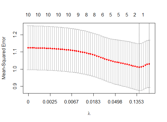
, (5) Equation (5) reduces to Equation (3), the conventional regression solution. As λ increases above zero, the penalty becomes increasingly dominant, which pushes the c coefficients toward zero (hence the name “shrinkage”). Those variables with zero coefficients will be removed from the model. Intuitively, it is the coefficients on the least important variables that are first pushed to zero, leaving the more important variables in the model to be estimated. (“Important” does not mean causal, but merely that it explains some of the variance of the historical data.)