Author Archives: Nikos

Temporal Big Data for Tire Industry Tactical Sales Forecasting

Y.R. Sagaert, E-H. Aghezzaf, N. Kourentzes and B. Desmet, 2017, Interfaces. https://doi.org/10.1287/inte.2017.0901

We propose a forecasting method to improve accuracy for tactical sales predictions at a major supplier to the tire industry. This level of forecasting serves as direct input for the demand planning, steering the global supply chain and is typically up to a year ahead. The case company has a product portfolio that is strongly sensitive to external events. Univariate statistical methods, which are common in practice, are unable to anticipate and forecast changes in the market, while human expert forecasts are known to be biased and inconsistent. The proposed method is able to automatically identify key leading indicators that drive sales from a massive set of macro-economic indicators, across different regions and markets and produce accurate forecasts. Our method is able to handle the additional complexity of the short and long term dynamics from the product sales and the external indicators. We find that accuracy is improved by 16.1% over current practice with proportional benefits for the supply chain. Furthermore, our method provides transparency to the market dynamics, allowing managers to better understand the events and economic variables that affect the sales of their products.

Download paper.

Can neural networks predict trended time series?

Yes and… no! First, I should say that I am thinking of the common types of neural networks that are comprised by neurons that use some type of sigmoid transfer function, although the arguments discussed here are applicable to other types of neural networks. Before answering the question, let us first quickly summarise how typical neural networks function. Note that the discussion is done in a time series forecasting context, so some of the arguments here are specific to that and are not relevant to classification tasks!

1. Multilayer Perceptron (MLP) neural networks

MLPs are a basic form of neural networks. Having a good understanding of these can help one understand most types of neural networks, as typically other types are constructed by adding more connections (such as feedbacks or skip-layer/direct connections). Let us assume that we have three different inputs, (X₁, X₂, X₃), which could be different variables or lags of the target variables. A MLP with a single hidden layer, with 5 hidden nodes and a single output layer can be visualised as in Fig. 1.

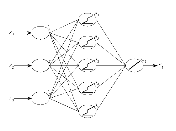
Fig. 1. MLP with 3 inputs, 5 hidden nodes arranged in a single layer and a single output node.

An input (for example X₁) is passed and processed through all 5 hidden nodes (H_i), the results of which are combined in the output (O₁). If you prefer, the formula is:
$Y_1 = b_0 + \sum_{i=1}^5 { \left( b_i f(a_{0,i} + \sum_{j=1}^3{a_{j,i}X_{j}}) \right) }$ , (1)
where b₀ and a_0,i are constants and b_i and a_j,i are weights for each input X_j and hidden node H_i. Looking carefully at either Eq. 1 or Fig. 1 we can observe that each neuron is a conventional regression that passes through a transfer function f() to become nonlinear. The neural network arranges several such neurons in a network, effectively passing the inputs through multiple (typically) nonlinear regressions and combining the results in the output node. This combination of several nonlinear regressions is what gives a neural network each approximation capabilities. With a sufficient number of nodes it is possible to approximate any function to an arbitrary degree of accuracy. Another interesting effect of this is that neural networks can encode multiple events using single binary dummy variables, as this paper demonstrates. We could add several hidden layers, resulting in a precursor to deep-learning. In principle we could make direct connections from the inputs to layers deeper in the network or the output directly (resulting in nonlinear-linear models) or feedback loops (resulting in recurrent networks).

The transfer function f() is typically either the logistic sigmoid or the hyperbolic tangent for regression problems. The output node typically uses a linear transfer function, acting as a conventional linear regression. To really understand how the input values are transformed to the network output, we need to understand how a single neuron functions.

2. Neurons

Consider a neuron as a nonlinear regression of the form (for the example with 3 inputs):

$H_i = f(a_{0,i} + \sum_{j=1}^3{a_{j,i}X_{j}})$ . (2)

If f() is the identity function, then (2) becomes a conventional linear regression. If f() is nonlinear then the magic starts! Depending on the values of the weights a_j,i and the constant a_0,i the behaviour of neuron changes substantially. To better understand this let us take the example of a single input neuron and visualise the different behaviours. In the following interactive example you can choose:

the type of transfer function;
the values of the input, weight and constant.

The first plot shows the input-output values, the plot of the transfer function and with cyan background the area of values that can be considered by the neuron given selected weight and constant. The second plot provides a view of the neuron function, given the transfer function, weight and constant. Observe that the weight controls the width of the neuron and the constant the location, along the transfer function.

What is quite important to note here is that both logistic sigmoid and hyperbolic tangent squash the input between two values and the output cannot increase or decrease indefinitely, as with the linear. Also the combination of weight and constant can result in different forms of nonlinearities or approximate linear behaviours. As a side note, although I do not see MLP as anything to do with simulating biological networks, the sigmoid-type transfer functions are partly inspired by the stimulated or not states of biological neurons.

By now two things should become evident:

The scale of the inputs is very important for neural networks, as very large or small values result in the same constant output, essentially acting at the bounds of the neuron plots above. Although in theory it is possible to achieve the desired scaling using only appropriate weights and constants, training of networks is aided tremendously by scaling the inputs to a reasonable range, often close to [-1,1].
With sigmoid type transfer functions it is impossible to achieve an ever increasing/decreasing range of outputs. So for example if we were to use as an input a vector (1, 2, 3, 4, 5, 6, …, n) the output would be squashed between [0, 1] or [-1, 1] depending on the transfer function, irrespectively of how large n is.

Of course, as Eq. (1) suggests, in a neural network the output of a neuron is multiplied by a weight and shifted by a constant, so it is relatively easy to achieve output values much greater than the bounds of a single neuron. Nonetheless, a network will still “saturate” and reach a minimum/maximum value and cannot decrease/increase perpetually, unless non-squashing neurons are used as well (this is for example a case where direct connections to a linear output become useful). An example of this follows.

Suppose we want to predict the future values of a deterministic upward trend with no noise, of the form: y_t = x_t and x_t = (1, 2, 3, 4, …). We scale the observed values between [-1, 1] to facilitate the training of the neural network. We use only 80% of the values for training the network and the remaining 20% to test the performance of the forecasts (test set A). We train a network with 5 logistic hidden nodes and a single linear output. Fig. 2 provides the resulting network with the trained weights and constants.

Fig. 2. Trained network for predicting deterministic trend.

The single input (scaled x_t) is fed to all five nodes. Observe that it is multiplied with different weights (black numbers) and shifted by different constants (blue numbers) at each node. When additional inputs are used, the inherent difficulty in interpreting all these weights together, makes neural networks to be considered as black boxes. Fig. 3 provides the observed y_t and predicted neural network values. The network is able to provide a very good fit in the training set and for most of test set A, but as the values increase (test set B) we can see that the networks starts to saturate (the individual nodes reach the upper bounds of the values they can output and eventually the whole network) and the predicted trend tapers off. As we saw earlier, each sigmoid-type node has a maximum value it can output.

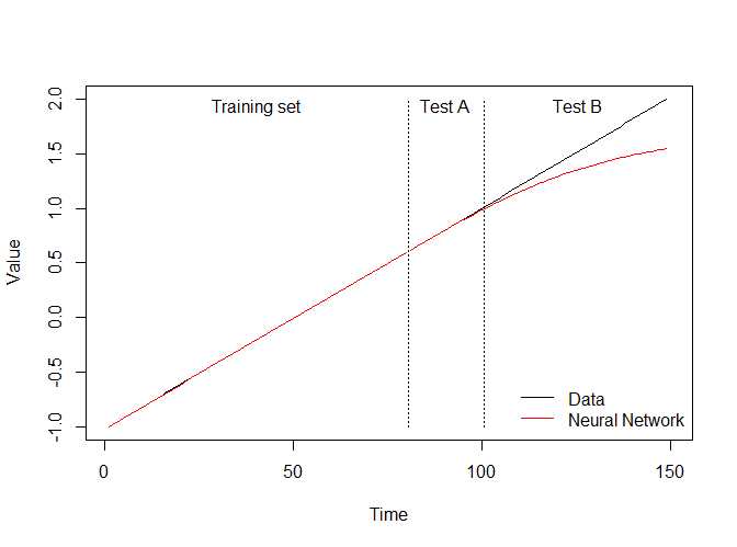
Fig. 3. Actuals and neural network values for the case of deterministic trend with no noise.

This raises a significant doubt whether neural networks can forecast trended time series, if they are unable to model such an easy case. One would argue that with careful scaling of data (see good fit in test set A) it is possible to predict trends, but that implies that one knows the range that the future values would be in, to accommodate them with appropriate scaling. This information is typically unknown, especially when the trend is stochastic in nature.

3. Forecasting trends

Although forecasting trends is problematic when using raw data, we can pre-process the time series to enable successful modelling. We can remove any trend through differencing. Much like with ARIMA modelling, we overcome the problem of requiring the network to provide ever increasing/decreasing values and therefore we can model such series. For example, considering one of the yearly M3 competition series we can produce the following forecast:

Fig. 4. Neural network forecast for a trending yearly M3 competition series.

Fig. 4 provides the actuals and forecasts after differencing and scaling is applied, the forecast is produced and subsequently differencing and scaling are reversed. However there are some limitations to consider:

This approach implies a two stage model, where first z_t= y_t– y_t-1is constructed and then z_t is modelled using neural networks. This imposes a set of modelling constraints that may be inappropriate.
The neural network is capable of capturing nonlinearities. However if such nonlinearities are connected to the level, for example multiplicative seasonality, then by using differences we are making it very difficult for the network to approximate the underlying functional form.
Differencing implies stochastic trend, which in principle is inappropriate when dealing with deterministic trend.

Therefore, it is fair to say that differencing is useful, but is by no means the only way to deal with trends and surely not always the best option. However, it is useful to understand how sigmoid-type neurons and networks are bound to fail in modelling raw trended time series. There have been several innovations in neural networks for forecasting, but most are bound by this limitation due to the transfer functions used.

So, can neural networks forecast trended time series? Fig. 4 suggests yes, but how to best do it is still an open question. Past research that I have been part of has shown that using differences is reliable and effective (for example see the specifications of neural networks here and here), even though there are unresolved problems with differencing. Surely just expecting the network to “learn” to forecasts trends is not enough.

Congratulations Dr. Svetunkov!

A couple of days ago it was the graduation ceremony for MSc and PhD students at Lancaster University. Ivan Svetunkov, one of my ex-PhD students officially graduated; well done Ivan! In a previous post I described briefly part of his research. He is also working on the excellent smooth package for R. You can find more about his work at his research blog. Also, well done to all the MSc graduates of the Dept. of Management Science, who had to survive my lectures!

The difference between in-sample fit and forecast performance

One of the fundamental differences in conventional model building, for example they way textbooks introduce regression modelling, and forecasting is how the in-sample fit statistics are used. In forecasting our focus is not a good description of the past, but a (hopefully) good prediction of the yet unseen values. One does not necessarily imply the other. A good fit does not necessarily lead to a good forecast, and vice-versa. For example, overfit models will typically have very small in-sample errors, but be terrible at forecasting. An example of the opposite case is shrinkage, where we sacrifice in-sample fit for good generalisation of the model.

A typical premise of forecasting model building is that a good fit in the past should lead to a reasonable forecast in the future. Implicitly we assume that there is some underlying data generating process, which we hopefully approximate well enough, to forecast it in the future. I do not believe that we can identify the true process for real data – I have come to doubt even if a true process exists, though this is a philosophical point. Here I will not make a discussion on how to avoid overfitting (for a related discussion see this post). Instead I will provide a slightly unusual example that I built for my students to exemplify the difference between in-sample fitting and forecasting.

For this example, I will not use a business time series, but music. We can extract from a song its waveform and analyse it as a time series, and even try to forecast it. There is a catch though, there is an inherent causality in music. It typically follows some logical structure, harmony and so on that a standard forecasting model is unaware of. For example, ARIMA or exponential smoothing, will attempt to find structure and repeating patterns in the past and extrapolate them in the future, unaware of any linguistics or musical constructs.

Let us take a song, sample its first 10 seconds, at 11,025 observations per second and fit an adequate ARIMA. Using standard unit root testing and AICc we identify an ARMA(5,0,4) as the best model. Note that the exact model used does not make much difference for this example, and different order ARIMA would provide more or less the same conclusions.

Using this model we forecast the next 5 seconds. We can assess the quality of the model fit and the forecast visually, but also as sound. Does the model fit sound anything like the original song? Does the forecast sound anything like the original song? Here it is a good point to warn you that I have chosen a sufficiently interesting song.

Fig. 1 provides a plot of the 1000 last historical observations and the ARMA fit, as well as the forecast for the next 500 observations, where we can easily evaluate the quality of the model fit.

Fig. 1. Plot of the 1000 last historical observations and model fit, as well as the next 500 forecasted periods.

We can observe that the model fit is relatively good, yet the forecast is very weak. In fact, the forecast quickly reverts to the mean and the prediction intervals “contain” all the song. This already makes it quite clear that a good fit does not mean a good forecast. The difference between the quality of the in-sample fit and the out-of-sample forecast is striking when “heard”.

The original sample:

The model fit:

The two sound samples are sufficiently similar. In fact, one can hear that the model fit is missing some of the higher pitches, which can be also seen in Fig. 1. Nonetheless, the fit sound sample is arguably retaining enough of the original song to be recognisable.

The forecast sounds like:

As seen in Fig. 1. the forecast very quickly becomes a flat line, which results in silence.

It is clear that although the model fit captures adequately the song, the forecast is useless. Why is this the case? The modelling methodology I followed here is geared towards good in-sample fit, rather than forecasting. Arguably the model family I used is also inappropriate. However, neither of these becomes apparent by consulting only the in-sample fit.

Generalising, consulting conventional in-sample statistics such as R², mean squared error, etc. is not only useless, but also dangerous, when the model building purpose is forecasting. Consulting penalised statistics, such as information criteria (AIC, BIC, etc.) is useful, but again care should be taken. In our example the best model was chosen using AICc and it still did not produce any useful forecast. Business forecasting is not that dissimilar from the example here.

The reason that forecasting fails here is that there was no consideration during model fitting to identify the key drivers of the time series, in this case the musical and linguistic structure (though there are no lyrics in the sample used here). Instead, a generic extrapolative model was used. Business series often have similar complexities, such as promotions, price changes, events, and so on. These should be part of the model building exercise. Simply flagging observations as outlying, or merely identifying and fitting the “best” model from a limited pool of alternatives is a dangerous strategy. What I often argue to my students is that a good modeller should appreciate the problem context and use it! In-sample statistics are woefully inadequate in doing this, especially when forecasting is the objective.

A final note: all rights for the song are with the original holders. I am in no way a composer myself and the song is not my work! Can anyone recognise which song it is?

Talk on `Advances in promotional modelling and demand forecasting’

On 16/11/2016 I gave a talk at the Stockholm School of Economics on the topic of advances in modelling and demand forecasting. Given the diversity of the audience I avoided going into the details of the mathematical formulations, some of which can be found in the appendix of the presentation. The presentation summarises three different research areas I have been active recently, with the help of colleagues and PhD students:

temporal aggregation and temporal hierarchies;
promotional modelling at SKU level;
use of online search data for lifecycle modelling.

You can download the slides here.

MAPAx available for R & new MAPA package on CRAN

The previous version of the MAPA package implemented only the univariate aspect of the algorithm. Version 2.0.1 implements MAPAx as well, which allows incorporating regressors in your forecasts. In this paper we demonstrated the usefulness of temporal aggregation in the case of forecasting demand in the presence of promotions. In particular, we showed that MAPAx substantially outperformed regression promotions models (of this type), as well as exponential smoothing with promotional information (see Fig. 1).

Fig. 1. Bias and accuracy results for heavily promoted items. Description and details of the case study and experiment can be found here.

To use MAPAx call the usual mapa functions with the addition of the argument xreg. You can also control whether the regressors are transformed using principal components or not, using the argument pr.comp. By default no transformation is performed. Note that MAPAx can only be used when type="es". It is recommended that when the regressors are related to high-frequency information, such as promotions, to use the combination options (argument comb): w.mean or w.median that weight high-frequency seasonality and xreg states more heavily.

The following example illustrates the strength of MAPAx when additional information is available. We model the demand of a promoted product with conventional MAPA and MAPAx. Fig. 2 provides the in-sample rolling forecasts and the out-of-sample forecast for 13 weeks.

Fig. 2. MAPA and MAPAx forecasts for the demand of a promoted product.

Observe that MAPAx models the past and future promotions and also provides tighter prediction intervals, since more information in the past sales is captured.

The stable version of the package with MAPAx is 2.0.1 and is available on CRAN. The development version, which includes the latest bugfixes, can be found on GitHub, where I also provide the versions available at both CRAN and GitHub so you can check whether you have the latest version or not. MAPAx, similar to high-frequency MAPA, requires the smooth package. Make sure you have the latest version of that as well!

MAPA package for R on GitHub

Here is the link: https://github.com/trnnick/mapa

It has been a long time I wanted to rework the MAPA package for R, but I could not find the time. Finally I got around starting it. There are three objectives in this:

Clean up code and introduce S3methods. MAPA was the first package that I wrote!
Incorporate the es exponential smoothing implementation from the smooth package. This is an alternative to ets that will remain as the default. It allows longer seasonal cycles and some additional customisation in the specification of the exponential smoothing models.
Implement MAPAx that permits introducting exogenous variables to MAPA.

Tidying up the code is an ever-ongoing process, so (1) will never finish! I have already sorted (2) out and the next task is to work on (3). You can grab the development version on GitHub. At the time of writing you will need the development version of smooth for this to work, on which Ivan has been ironing out a few peculiar bugs that MAPA brought to surface. You will be amazed how much temporal aggregation can mess up otherwise stable code!

Here is a sneak peak of things you could not do with MAPA before:

mapafit <- mapaest(taylor,ppy=336,type="es")
plot(mapafit)

Fig. 1: Look at all these aggregation levels!

The new argument is type="es" that lets MAPA know what exponential smoothing implementation to use. Once the estimation is done we can use this to forecast as usual.

mapacalc(taylor,mapafit,comb="wght",outplot=2)

Fig. 2: MAPA for high frequency data!

So finally we can now easily use MAPA for series with seasonality more than 24 periods! You may have observed that I am using a different combination of the temporal aggregation states: wght. This is still experimental, so use it at your own risk! I would still recommend using either median or mean.

Another nice feature that the es implementation offers is more flexibility in specifying models. Before we could use the model="ZZZ" to let ets select the best model for each aggregation level. Now we can use the letters X and Y to restrict the search to only additive or multiplicative options (including N) respectively. So for example we could set model="ZXA" to have MAPA look for exponential smoothing models with any type of error, trend that can be none, additive or damped additive and additive seasonality.

Which of ets or es is most accurate to use with MAPA? This is a difficult question to answer. In different examples I tried, I got different results, but there are a few things I can point out. ets from the forecast package by default does not allow multiplicative trends. This was done as using only additive trends seems to work better for ets. This is not the case for es that considers all possible trends. In the current MAPA implementation you can use the argument allow.multiplicative.trend=TRUE to make ets consider all trends. Similarly, with es you can use model="ZXZ" to restrict it to additive trends. On the M3 dataset, once the specification is identical (only additive trends) es based MAPA performs about 5% worse than ets based MAPA, which is fairly small difference, with no evidence of statistically significant differences. So my recommendation is as follows: MAPA with ets works fine and is the default core, but if the additional flexibility of es is needed, feel confident in using it!

Complex Exponential Smoothing

A couple of days ago my ex-student Ivan Svetunkov successfully defended his PhD. My thanks to both Siem Jan Koopman and Rebecca Killick who were his examiners and with their questions led to a very interesting discussion.

Ivan’s PhD topic is a new model, the Complex Exponential Smoothing (CES). In this post I will very briefly demonstrate the key advantages of the proposed model over conventional exponential smoothing. I will not go into the mathematical details, which can be found in detail in this working paper. Furthermore, a CES implementation is available in the smooth package for R.

One of the motivating ideas behind CES is that recent research has demonstrated that the standard forms of exponential smoothing may not be able to capture all the patterns observed in real time series. In particular, the interpretation of the level and trend components, once one goes in the details, is elusive and arguably the distinction is ad-hoc, perhaps leading to more modelling woes than what it solves. Instead, CES avoids this separation, and introduces a new flexible component that captures various types of information, beyond the level component, as necessary to achieve good fit to the given data.

Effectively, CES is able to model a wide spectum of level and trend time series, without requiring to switch between different models, as is the case for exponential smoothing. CES is able to model both stationary and non-stationary in the mean time series, whereas exponential smoothing is capable of modelling only non-stationary ones. Because CES does not switch between level and trend models, but smoothly “slides” between the two types, not only it captures more behaviours, but also avoids any abrupt changes in successive forecasts of a time series. For example, as new data become available and new forecasts are generated, a different form of exponential smoothing may become optimal, for instance using Akaike Information Criterion, and new forecasts may become substantially different. In turn, this may cause issues for the users of the forecasts, as they become very erratic. The Multiple Prediction Aggregation Algorithm (MAPA) addressed this by strengthening the identification and estimation of exponential smoothing, but at the cost of multiple model fits. CES does that by proposing an alternative the modelling series as if they are separable into level and trend components.

The following example illustrates the point. I have simulated a simple exponential smoothing (level) and a Holt linear trend exponential smoothing (trend) time series. Both time series are 8 years long (96 monthly observations). For the last 4 years I perform a rolling origin evaluation experiment. At each forecast origin models are optimised and appropriate forecasts are produced. The fitting sample is extended by one observation and the process is repeated, until there is no remaining sample. At minimum 4 years of data are used to fit the first batch of models. Fig. 1 and Fig. 2 visualise the process for the level and trend series respectively.

Fig. 1: CES and ETS rolling forecasts on test set for the level time series.

Fig. 2: CES and ETS rolling forecasts on test set for the trend time series.

Observe the erratic changes in the forecasts in the ETS case. These are caused by switching between level and trend models, which are not always correctly identified. For the level series the misspecification occurs 32% of the times, whereas for the trend series 24%. The figures provide the avergae Mean Absolute Error (MAE) across forecast origins, showing that CES is more accurate. Of course, these are just two examples, and I refer you to the working paper for a more rigorous evaluation of CES.

An advantage of CES is that it sidesteps model selection. The same model is adequate for both level and trend series. This is not possible with conventional time series models. We argue that this simplifies the forecasting process substantially, both in terms of complexity and computational requirements. Fig. 3 illustrates the point by providing the total computation time for each example above. ETS requires substantially more time, as 19 different models are trialed at each forecast origin.

Fig. 3: Total computation time for each example.

Ivan looked into the properties of the basic CES model, deriving likelihood, parameter bounds and variance expressions. He then proceeded to extend the model to the seasonal case. The conventional repertoire of series that exponential smoothing models is tackled by only two variants of CES: non-seasonal and seasonal, retaining the model selection challenge relatively simple. Obviously, we do not claim dominance of CES over ETS in every case, but the empirical results are favourable to CES, especially when the qualitative elements of the comparison (simplified or no model selection) are considered. Detailed results are descriptions are in two papers currently under review, which I hope I will be able to post here soon. Meanwhile there are two presentations by Ivan that you may find helpful about CES and seasonal CES.

If you want to trial CES for yourselves, I recommend you to explore the smooth package for R that is available on CRAN.

Finally, let me congratulate Ivan for successfully defending his PhD!

TStools recent changes

We have been re-working the TStools package over the past couple of weeks. The major changes are:

The es function that is an alternative to the ets function from the forecast package has been removed. Now it is published separately in the smooth package, which contains a collection of interesting implementations for exponential smoothing, ARIMA and more novel forecasting algorithms such as the Complex Exponential Smoothing that Ivan Svetunkov (the author of the package) and I have been working on. You can read more about the benefits of es function and the package at his blog.
Re-worked the nemenyi function to streamline the inputs and outputs, as well as improve the visualisation for the MCB test. Now the figure highlights methods for which there is insufficient evidence of differences.
Inspired by my recent blog post on ABC-XYZ analysis, I re-coded the functions abc, xyz and abcxyz. They are now much more flexible in terms of plotting, accepting arguments for the plot function. When none are provided the functions revert to default behaviour. Furthermore, I got rid of the colouring using transparencies, which caused a few issues wen exporting figures in specific formats. Finally, the abcxyz function now accepts an additional input argument. Now, you can provide a vector of forecast errors which will be average for each class and reported as an array and in the plot. This is quite handy for easily tracking forecasting performance per class. The following figure provides an example.

The top number reports the number of items in each class and the lower the average error.

Research visit at Stockholm School of Economics

I started this month my sabbatical leave and I am currently visiting the Center for Economic Statistics at the Stockholm School of Economics until the end of December, 2016. My thanks to Rickard Sandberg, who is hosting me and is also the director of the centre. The focus of our research will be on business forecasting and more particularly looking at hierarchical aspects of it.

Related Posts

Related Posts

Related Posts

Related Posts

Related Posts

Related Posts

Related Posts

Related Posts

Related Posts